Aerobatic flight. Part 2. The simplest model of movement to perform the barrel
We continue a series of articles on the automation of performing aerobatic flying on a small RPV. This article has, above all, an educational goal: here we will show how you can create the simplest automatic control system (ACS) using the example of performing the “barrel” aerobatic operation while controlling an aircraft only with ailerons. The article is the second in the series of publications “Piloting RPV”, which tells about the process of building hardware and software parts of ACS in a training form.

Link to the previous article of the cycle:
1. “Aerobatic RPV. How to make a barrel "
Introduction
Motion Model Model
Parameters. Moment of inertia
Model parameters. Derivatives of moment of roll.
Verification of the model.
Synthesis of control for performing the “barrel”
Flight experiment
Remarks
Conclusions
So, we decided to implement the "barrel" in automatic mode. It is obvious that for the automatic execution of the figure it is necessary to formulate the corresponding control law. The process of inventing will be much more painless and faster if you use the mathematical model of the movement of the aircraft. Testing the control law in the flight experiment is possible, but it takes much longer, and it can be much more expensive in case of loss or damage to the vehicle.
Since at low angles of attack and gliding of the aircraft, its movement along the roll is practically unrelated to movement in two other channels: traveling and longitudinal - to perform a simple “barrel” it will be enough to build a model of movement only around one axis - OX axis of the connected SC. For the same reason, the aileron control law will not change significantly when it comes to creating a complete control system.
The equation of motion of the aircraft around the longitudinal axis OX of the connected SC is extremely simple: - moment of inertia about axis OX , and moment
 consists of several components, of which for a realistic description of the movement of our aircraft, it is enough to consider only two:
  - the moment due to the rotation of the aircraft around the axis OX (damping moment),
 - the moment due to the deviation of the ailerons (control torque). The last expression is written in linearized form: moment of roll linearly dependent on angular velocity
  and aileron deflection angle
  with constant coefficients of proportionality
  and
and  respectively.
As is known (for example, from Wiki ), a linear differential equation - Transmission function,
  - operator differentiation
  - time constant, and
  - gain.
For aperiodic link time constant equal to the time for which the output value  with a single step effect of input value
  takes a value that differs from the steady state by ~ 5%, and the gain numerically equal to the steady-state value of the output value with a single step effect:

In the constructed motion model, there are two unknown parameters: the gain and time constant . These parameters are expressed through the characteristics of the physical system: moment of inertia, as well as the derivatives of the moment of roll and :
then, by defining the parameters of the model, it is possible to restore the system parameters from them.
Model parameters. Moment of inertia
Our aircraft consists of the following parts: wing, fuselage with tail, engine, battery (battery) and avionics :

The avionics include: autopilot board, SNS receiver board, radio modem board, control signal receiver board, two speed regulators motor and connecting wires.

Due to the low weight of the avionics, its contribution to the total moment of inertia can be neglected.
The total value of the moment of inertia of the aircraft with respect to the axis OX is obtained by adding the moments of inertia of the parts:, it turned out the following:
It is seen that the main contribution to the total moment of inertiamakes the wing. This is due to the fact that the wing has a fairly large transverse size (wing span - 1 m):

Therefore, despite the modest weight (about 20% of the total take-off weight of the aircraft), the wing has a significant moment of inertia.
Model parameters. Derivatives of moment roll
The calculation of the derivatives of the moment of roll is a rather difficult task associated with the calculation of the aerodynamic characteristics of the aircraft by numerical methods or using engineering techniques. The application of the first and second requires significant time, intellectual and computational costs, which are justified in the development of control systems for large aircraft, where the cost of the error still exceeds the cost of building a good model. For the task of controlling a UAV, whose mass does not exceed 2 kg, this approach is hardly justified. Another way to calculate these derivatives is flight experiment. Given the cheapness of our aircraft, as well as the proximity of a suitable field for such an experiment, the choice was obvious for us.
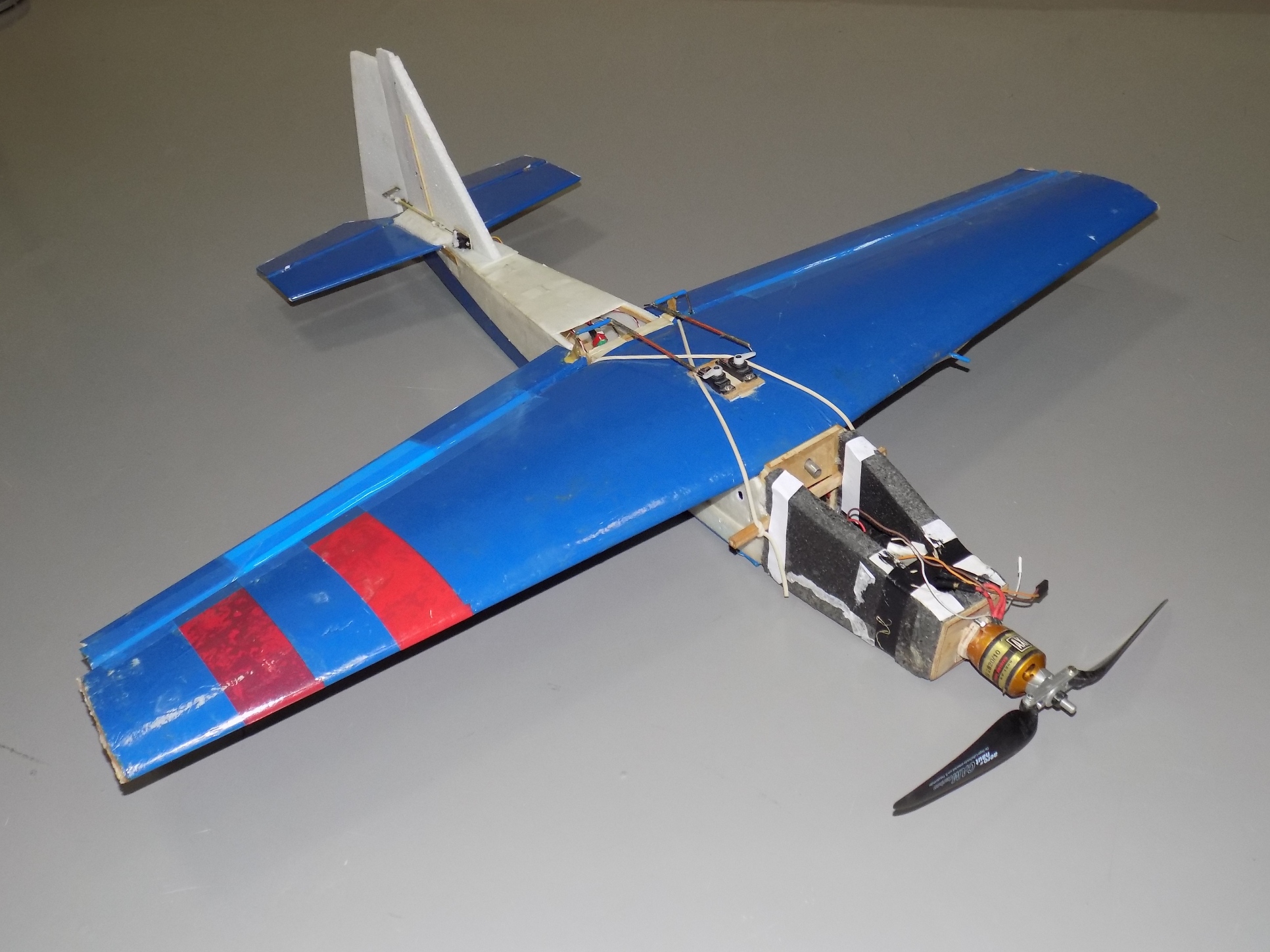
Writing into the autopilot firmware for manual control and registration of parameters, we assembled the aircraft and prepared it for testing:
In the flight experiment, we managed to obtain data on the aileron deflection angle and the angular velocity of the aircraft rotation. The pilot operated the aircraft in manual mode, flying in a circle, turning and “barrels”, and the onboard equipment recorded and sent the necessary information to the ground station. As a result, the necessary dependencies were obtained: (degrees / s) and (b / r). Magnituderepresents the normalized deflection angle of ailerons: the value 1 corresponds to the maximum deviation, and the value −1 to the minimum:

How now to determine and from the data? The answer is to measure the parameters of the transition process according to the graphs. and .
The result of determining the values of the time constant and the gain is as follows: ,
,  . These values of the coefficients at a known value of the moment of inertia The following values of the derivatives of the moment of roll correspond:
So, building a model, the basis of which is an aperiodic link obtained from the flight experiment, and compare the output signal of the model with the value , also obtained in the experiment.
The result of the verification is shown in the figure:

As can be seen from the figure, the coincidence of the model with reality is slightly less than complete.
Having obtained the model, it is easy to determine by what amount and for how long it is necessary to reject the ailerons in order to perform the “barrel”. One option is the following deviation algorithm:

The presence of segments with a duration of 0.1 s at the beginning and at the end of the aileron deflection algorithm models the inertia of the servo, which cannot deflect surfaces instantly. The model shows that with such a law, the deviations of the ailerons of the aircraft should perform one complete revolution around the axis OX , will we check?
The resulting aileron control law was programmed into the autopilot installed on the aircraft. The idea of the experiment is simple: bring the plane to horizontal flight, and then use the resulting control law. If the actual movement of the aircraft along the roll corresponds to the model created, the aircraft must perform a “barrel” - one full turn at 360 degrees.
Separately, we express our gratitude to our faithful pilot for his work, professionalism and comfortable trunk on Priore-wagon!
In the course of the experiment, it became clear that the roll motion model was built successfully - the aircraft performed one “barrel” after another, as soon as the pilot activated the programmed control law. The following figure shows the angular velocity.recorded during the experiment, and obtained from the simulation results, as well as the roll and pitch angle from the flight experiment:

And the following figure shows the signals recorded in the flight experiment on ailerons, elevator (RV) and rudder (PH):

Vertical lines are indicated moments of the beginning and end of the "barrel". From the figures it is clear that in the process of performing the “barrel” the pilot does not interfere with the control of the elevator and the rudder. in the flight simulator (see the article "Aerobatic RPV. How to make a barrel correctly"). If you carefully review the previous graphs, it will become clear that the third “barrel” was not even finished, because the pilot intervened in control to take the plane out of a dive: the pitch angle changes so much when performing “barrels” with ailerons alone.
As a result of the work we have done, we showed one of the ways to create a model of RPV motion using the angular velocity. In the flight experiment it was proved that the created model of movement fully corresponds to the simulated object. On the basis of the developed model, the law of software control was obtained, which allows to perform the “barrel” in the automatic mode. We also made sure that it would not be possible to execute the correct “barrel” with the ailerons alone, and also demonstrated this clearly.
The next step will be the refinement of the control law by adding feedback, and the inclusion of the elevator in the control. The latter will require the creation of a model of the longitudinal movement of our aircraft. The results of the work will be the next publication.
Link to the previous article of the cycle:
1. “Aerobatic RPV. How to make a barrel "
Content:
Introduction
Motion Model Model
Parameters. Moment of inertia
Model parameters. Derivatives of moment of roll.
Verification of the model.
Synthesis of control for performing the “barrel”
Flight experiment
Remarks
Conclusions
Introduction
So, we decided to implement the "barrel" in automatic mode. It is obvious that for the automatic execution of the figure it is necessary to formulate the corresponding control law. The process of inventing will be much more painless and faster if you use the mathematical model of the movement of the aircraft. Testing the control law in the flight experiment is possible, but it takes much longer, and it can be much more expensive in case of loss or damage to the vehicle.
Since at low angles of attack and gliding of the aircraft, its movement along the roll is practically unrelated to movement in two other channels: traveling and longitudinal - to perform a simple “barrel” it will be enough to build a model of movement only around one axis - OX axis of the connected SC. For the same reason, the aileron control law will not change significantly when it comes to creating a complete control system.
Motion Model
The equation of motion of the aircraft around the longitudinal axis OX of the connected SC is extremely simple:

- moment of inertia about axis OX , and moment consists of several components, of which for a realistic description of the movement of our aircraft, it is enough to consider only two: 
- the moment due to the rotation of the aircraft around the axis OX (damping moment),- the moment due to the deviation of the ailerons (control torque). The last expression is written in linearized form: moment of roll linearly dependent on angular velocity and aileron deflection angle with constant coefficients of proportionality and respectively. As is known (for example, from Wiki ), a linear differential equation


- Transmission function, - operator differentiation - time constant, and - gain.How to move from a differential equation to a transfer function?
In our case, from the parameters of the equation to the parameters of the transfer function, you can go as follows (knowing that the derivative negative):
negative):


For aperiodic link time constant
equal to the time for which the output value with a single step effect of input value takes a value that differs from the steady state by ~ 5%, and the gain numerically equal to the steady-state value of the output value with a single step effect:In the constructed motion model, there are two unknown parameters: the gain
and time constant . These parameters are expressed through the characteristics of the physical system: moment of inertia, as well as the derivatives of the moment of roll and :
then, by defining the parameters of the model, it is possible to restore the system parameters from them.Model parameters. Moment of inertia
Our aircraft consists of the following parts: wing, fuselage with tail, engine, battery (battery) and avionics :
The avionics include: autopilot board, SNS receiver board, radio modem board, control signal receiver board, two speed regulators motor and connecting wires.
Due to the low weight of the avionics, its contribution to the total moment of inertia can be neglected.
How was the estimation of the moment of inertia?
Estimation of the moment of inertia can be carried out as follows. Let's look at the plane along the axis OX :

And then we will present it in the form of the following simplified model:

Scheme for calculating the moment of inertia. Top left - the battery, bottom right - the engine. The engine and battery are located on the axis of the fuselage.
It can be seen that for the creation of the model, the keel, horizontal tail, propeller, and avionics were rejected. At the same time left: the fuselage, wing, battery, engine. By measuring the masses and characteristic dimensions of each part, it is possible to calculate the moments of inertia of each part relative to the longitudinal axis of the fuselage:
can be carried out as follows. Let's look at the plane along the axis OX : And then we will present it in the form of the following simplified model:
Scheme for calculating the moment of inertia
. Top left - the battery, bottom right - the engine. The engine and battery are located on the axis of the fuselage.It can be seen that for the creation of the model, the keel, horizontal tail, propeller, and avionics were rejected. At the same time left: the fuselage, wing, battery, engine. By measuring the masses and characteristic dimensions of each part, it is possible to calculate the moments of inertia of each part relative to the longitudinal axis of the fuselage:
- wing (thin rod):

- fuselage (hollow cylinder):

- battery (plate):

- engine (drive):

The total value of the moment of inertia of the aircraft with respect to the axis OX is obtained by adding the moments of inertia of the parts:

, it turned out the following:- wing - 96.3%,
- fuselage - 1.6%,
- engine and battery - 2%,
It is seen that the main contribution to the total moment of inertia
makes the wing. This is due to the fact that the wing has a fairly large transverse size (wing span - 1 m): Therefore, despite the modest weight (about 20% of the total take-off weight of the aircraft), the wing has a significant moment of inertia.
Model parameters. Derivatives of moment roll and
The calculation of the derivatives of the moment of roll is a rather difficult task associated with the calculation of the aerodynamic characteristics of the aircraft by numerical methods or using engineering techniques. The application of the first and second requires significant time, intellectual and computational costs, which are justified in the development of control systems for large aircraft, where the cost of the error still exceeds the cost of building a good model. For the task of controlling a UAV, whose mass does not exceed 2 kg, this approach is hardly justified. Another way to calculate these derivatives is flight experiment. Given the cheapness of our aircraft, as well as the proximity of a suitable field for such an experiment, the choice was obvious for us.
Writing into the autopilot firmware for manual control and registration of parameters, we assembled the aircraft and prepared it for testing:
In the flight experiment, we managed to obtain data on the aileron deflection angle and the angular velocity of the aircraft rotation. The pilot operated the aircraft in manual mode, flying in a circle, turning and “barrels”, and the onboard equipment recorded and sent the necessary information to the ground station. As a result, the necessary dependencies were obtained:
(degrees / s) and (b / r). Magnituderepresents the normalized deflection angle of ailerons: the value 1 corresponds to the maximum deviation, and the value −1 to the minimum: How now to determine
and from the data? The answer is to measure the parameters of the transition process according to the graphs. and .How were the k and T coefficients determined?
Gain determined by assigning values of steady-state value of the angular velocity to a value aileron deflection:

Dependence of the deflection angle of the ailerons and roll rate of the time obtained in lotnom experiment
the previous figure plots the steady values of the angular speed of approximately correspond to, e.g., the segments near the time points 422, 425 and 438 with (marked in dark red in the picture).
Time constantdetermined from the same graphs. For this, areas of abrupt change of the aileron deflection angle were found, and then the time was taken during which the angular velocity takes a value that differs from the steady-state value by 5%.
determined by assigning values of steady-state value of the angular velocity to a value aileron deflection: Dependence of the deflection angle of the ailerons and roll rate of the time obtained in lotnom experiment
the previous figure plots the steady values of the angular speed of approximately correspond to, e.g., the segments near the time points 422, 425 and 438 with (marked in dark red in the picture).
Time constant
determined from the same graphs. For this, areas of abrupt change of the aileron deflection angle were found, and then the time was taken during which the angular velocity takes a value that differs from the steady-state value by 5%.The result of determining the values of the time constant and the gain is as follows:
, . These values of the coefficients at a known value of the moment of inertia The following values of the derivatives of the moment of roll correspond:![$ M_x ^ {\ omega_x} = - \ frac {I_x} {T} = - 0.24 \ frac {\ text {N} \ cdot \ text {m}} {\ text {deg / s}}, {\ color { white} \ longrightarrow} M_x ^ {\ delta_a} = - kM_x ^ {\ omega_x} = \ frac {kI_x} {T} = - 138 \ frac {\ text {N} \ cdot \ text {m}} {\ text {[]}}. $](https://habrastorage.org/getpro/geektimes/formulas/5fe/389/b33/5fe389b33a7ca88a4a2129de715a022d.svg)
Model verification
So, building a model, the basis of which is an aperiodic link

obtained from the flight experiment, and compare the output signal of the model with the value , also obtained in the experiment.How was the simulation?
Инструмент для проведения моделирования мы выбирали, прежде всего, основываясь на возможности повторения результатов широким кругом читателей: это прежде всего означает, что программа должна быть в общественном доступе. В принципе задачу моделирования поведения апериодического звена первого порядка можно решить и создав свой собственный инструмент с нуля. Но так как в дальнейшем модель будет усложняться, то создание своего инструмента может отвлечь от основной задачи — создания САУ пилотажного ДПЛА. С учётом принципа открытости инструмента мы выбрали JSBsim.
В предыдущем разделе мы получили значения коэффициентов и . Используем их для моделирования движения самолета. Из прошлой статьи мы помним, что конфигурация модели самолета в JSBsim задается при помощи XML файла. Создадим собственную модель:
Так как мы строим модель движения аппарата только по крену, оставим многие из секций файла пустыми. В файле модели последовательно задаются следующие характеристики.
Геометрические размеры самолёта задаются в секции metrics: площадь крыла, размах, длина средней аэродинамической хорды, площадь горизонтального оперения, плечо горизонтального оперения, площадь вертикального оперения, плечо вертикального оперения, положение аэродинамического фокуса.
Массовые характеристики самолёта задаются в секции mass_balance: тензор инерции самолета, вес пустого самолета, положение центра масс.
Стоит отметить, что абсолютные положения аэродинамического фокуса и центра масс самолета не участвуют в расчете динамики аппарата, важно их относительное расположение.
Далее следуют секции, описывающие характеристики шасси самолета и его силовой установки.
В следующей секции, ответственной за систему управления, заполним канал, ответственный за управление по крену: укажем единственный вход fcs/aileron-cmd-norm, величина которого будет нормирована от -1 до 1.
Аэродинамические характеристики задаются в секции aerodynamics: силы задаются в скоростной системе координат, моменты — в связанной. Нас интересует момент по крену. В секции axis name=«ROLL» задаются функции, которые определяют момент сил от различных составляющих проекции момента аэродинамических сил на ось OX связанной системы координат. В нашей модели таких составляющих две. Первая составляющая — демпфирующий момент, который равен произведению угловой скорости на определенный ранее коэффициент. Вторая составляющая — это момент от элеронов при фиксированной скорости полёта: он равен произведению ранее определенного коэффициента на величину отклонения элеронов.
Стоит отметить, что при определении коэффициента была использована размерная величина . В наших полетных данные величина угловой скорости измерялась в градусах в секунду, тогда как в JSBSim используются радианы в секунду, поэтому коэффициент должен быть приведен к нужной нам размерности, т. е. разделен на 180 градусов и умножен на  радиан. Записываем эти составляющие момента аэродинамических сил внутри функций произведения product. При моделировании результат выполнения всех функций суммируется и получается значение проекции аэродинамического момента на соответствующую ось.
Проверить созданную модель можно на экспериментальных данных, полученных при лётных испытаниях. Для этого создаем скрипт следующего содержания:
where dots indicate missing data. In the file of the script familiar to us from the previous article, a new type of event ( “Time Notif” ) has appeared, which allows setting a continuous change of the parameter in time. The dependence of the parameter on time is given by a table function. JSBSim linearly interpolates the value of a function between tabular data. The verification procedure of the roll motion model consists in the execution of this script on the created model and comparing the results with the experimental ones.
В предыдущем разделе мы получили значения коэффициентов
и . Используем их для моделирования движения самолета. Из прошлой статьи мы помним, что конфигурация модели самолета в JSBsim задается при помощи XML файла. Создадим собственную модель:<?xml version="1.0"?><fdm_configname="OP1"version="2.0"release="BETA"><metrics><wingareaunit="M2"> 0.2 </wingarea><wingspanunit="M"> 1.0 </wingspan><chordunit="M"> 0.2 </chord><htailareaunit="M2"> 0.03 </htailarea><htailarmunit="M"> 0.5 </htailarm><vtailareaunit="M2"> 0.03 </vtailarea><vtailarmunit="M"> 0.5 </vtailarm><locationname="AERORP"unit="M"><x> -0.025 </x><y> 0 </y><z> 0.05 </z></location></metrics><mass_balance><ixxunit="KG*M2"> 0.018 </ixx><iyyunit="KG*M2"> 0.018 </iyy><izzunit="KG*M2"> 0.018 </izz><emptywtunit="KG"> 1.2 </emptywt><locationname="CG"unit="M"><x> 0 </x><y> 0 </y><z> 0 </z></location></mass_balance><ground_reactions></ground_reactions><propulsion></propulsion><flight_controlname="FCS: OP1"><channelname="Pitch"></channel><channelname="Roll"><summername="Roll Trim Sum"><input>fcs/aileron-cmd-norm</input><clipto><min>-1</min><max>1</max></clipto></summer></channel><channelname="Yaw"></channel></flight_control><aerodynamics><axisname="DRAG"></axis><axisname="SIDE"></axis><axisname="LIFT"></axis><axisname="ROLL"unit="N*M"><functionname="aero/coefficient/Clp"><description>Roll_moment_due_to_roll_rate</description><product><property>velocities/p-aero-rad_sec</property><value>-0.24</value></product></function><functionname="aero/coefficient/Clda"><description>Roll_moment_due_to_aileron</description><product><property>fcs/aileron-cmd-norm</property><value> 2.4 </value></product></function></axis><axisname="PITCH"></axis><axisname="YAW"></axis></aerodynamics><outputname="OP1.csv"rate="60"type="CSV"><property> velocities/vc-kts </property><property> aero/alphadot-deg_sec </property><property> aero/betadot-deg_sec </property><property> fcs/throttle-cmd-norm </property><simulation> OFF </simulation><atmosphere> OFF </atmosphere><massprops> OFF </massprops><aerosurfaces> ON </aerosurfaces><rates> ON </rates><velocities> ON </velocities><forces> OFF </forces><moments> OFF </moments><position> ON </position><coefficients> OFF </coefficients><ground_reactions> OFF </ground_reactions><fcs> ON </fcs><propulsion> OFF </propulsion></output></fdm_config>Так как мы строим модель движения аппарата только по крену, оставим многие из секций файла пустыми. В файле модели последовательно задаются следующие характеристики.
Геометрические размеры самолёта задаются в секции metrics: площадь крыла, размах, длина средней аэродинамической хорды, площадь горизонтального оперения, плечо горизонтального оперения, площадь вертикального оперения, плечо вертикального оперения, положение аэродинамического фокуса.
Массовые характеристики самолёта задаются в секции mass_balance: тензор инерции самолета, вес пустого самолета, положение центра масс.
Стоит отметить, что абсолютные положения аэродинамического фокуса и центра масс самолета не участвуют в расчете динамики аппарата, важно их относительное расположение.
Далее следуют секции, описывающие характеристики шасси самолета и его силовой установки.
В следующей секции, ответственной за систему управления, заполним канал, ответственный за управление по крену: укажем единственный вход fcs/aileron-cmd-norm, величина которого будет нормирована от -1 до 1.
Аэродинамические характеристики задаются в секции aerodynamics: силы задаются в скоростной системе координат, моменты — в связанной. Нас интересует момент по крену. В секции axis name=«ROLL» задаются функции, которые определяют момент сил от различных составляющих проекции момента аэродинамических сил на ось OX связанной системы координат. В нашей модели таких составляющих две. Первая составляющая — демпфирующий момент, который равен произведению угловой скорости на определенный ранее коэффициент
. Вторая составляющая — это момент от элеронов при фиксированной скорости полёта: он равен произведению ранее определенного коэффициента на величину отклонения элеронов.Стоит отметить, что при определении коэффициента
была использована размерная величина . В наших полетных данные величина угловой скорости измерялась в градусах в секунду, тогда как в JSBSim используются радианы в секунду, поэтому коэффициент должен быть приведен к нужной нам размерности, т. е. разделен на 180 градусов и умножен на радиан. Записываем эти составляющие момента аэродинамических сил внутри функций произведения product. При моделировании результат выполнения всех функций суммируется и получается значение проекции аэродинамического момента на соответствующую ось.Проверить созданную модель можно на экспериментальных данных, полученных при лётных испытаниях. Для этого создаем скрипт следующего содержания:
<?xml version="1.0" encoding="utf-8"?><runscript><useaircraft="ownPlane1"initialize="scripts/airborne"/><runstart="0"end="51"dt="0.01"><eventname="Trims"><condition> sim-time-sec ge 0.0 </condition><setname="simulation/do_simple_trim"value="5"/></event><eventname="Time Notif"continuous="true"><description>Provide a time history input for the aileron</description><condition> sim-time-sec ge 0</condition><setname="fcs/aileron-cmd-norm" ><function><table><independentVarlookup="row">sim-time-sec</independentVar><tableData>
0	0.00075
0.1	0.00374
0.2	-0.00075
0.3	-0.00075
0.4	-0.00075
0.5	-0.00075
0.6	0.00075
0.7	0.00075
...
48.8	-0.00075
48.9	0.00000
49	-0.00075
	</tableData></table></function></set></event></run></runscript>
where dots indicate missing data. In the file of the script familiar to us from the previous article, a new type of event ( “Time Notif” ) has appeared, which allows setting a continuous change of the parameter in time. The dependence of the parameter on time is given by a table function. JSBSim linearly interpolates the value of a function between tabular data. The verification procedure of the roll motion model consists in the execution of this script on the created model and comparing the results with the experimental ones.
The result of the verification is shown in the figure:
As can be seen from the figure, the coincidence of the model with reality is slightly less than complete.
Synthesis of control to perform the "barrel"
Having obtained the model, it is easy to determine by what amount and for how long it is necessary to reject the ailerons in order to perform the “barrel”. One option is the following deviation algorithm:
 : ailerons begin to deviate from the neutral position;
 : ailerons rejected by 50%;
 : ailerons begin to deviate to the neutral position;
 : ailerons in neutral.
The presence of segments with a duration of 0.1 s at the beginning and at the end of the aileron deflection algorithm models the inertia of the servo, which cannot deflect surfaces instantly. The model shows that with such a law, the deviations of the ailerons of the aircraft should perform one complete revolution around the axis OX , will we check?
Flight experiment
The resulting aileron control law was programmed into the autopilot installed on the aircraft. The idea of the experiment is simple: bring the plane to horizontal flight, and then use the resulting control law. If the actual movement of the aircraft along the roll corresponds to the model created, the aircraft must perform a “barrel” - one full turn at 360 degrees.
Separately, we express our gratitude to our faithful pilot for his work, professionalism and comfortable trunk on Priore-wagon!
In the course of the experiment, it became clear that the roll motion model was built successfully - the aircraft performed one “barrel” after another, as soon as the pilot activated the programmed control law. The following figure shows the angular velocity.
recorded during the experiment, and obtained from the simulation results, as well as the roll and pitch angle from the flight experiment: And the following figure shows the signals recorded in the flight experiment on ailerons, elevator (RV) and rudder (PH):
Vertical lines are indicated moments of the beginning and end of the "barrel". From the figures it is clear that in the process of performing the “barrel” the pilot does not interfere with the control of the elevator and the rudder. in the flight simulator (see the article "Aerobatic RPV. How to make a barrel correctly"). If you carefully review the previous graphs, it will become clear that the third “barrel” was not even finished, because the pilot intervened in control to take the plane out of a dive: the pitch angle changes so much when performing “barrels” with ailerons alone.
Remarks
- Built ACS to perform the "barrel" does not take into account the dependence of the derivatives of the moment of the roll on the flight speed. On the one hand, this was done in order not to complicate the model and the law of control. On the other hand, such a dependence is easy to introduce if instead of derivatives and use quantities
 and
and  determined at a given flight speed
  .
. - The developed control law is a program control without feedback. The presence of feedback on the angular velocity and / or roll angle will improve the accuracy of the figure, which will be done in the future.
findings
As a result of the work we have done, we showed one of the ways to create a model of RPV motion using the angular velocity
. In the flight experiment it was proved that the created model of movement fully corresponds to the simulated object. On the basis of the developed model, the law of software control was obtained, which allows to perform the “barrel” in the automatic mode. We also made sure that it would not be possible to execute the correct “barrel” with the ailerons alone, and also demonstrated this clearly. The next step will be the refinement of the control law by adding feedback, and the inclusion of the elevator in the control. The latter will require the creation of a model of the longitudinal movement of our aircraft. The results of the work will be the next publication.