Building orbits of celestial bodies using Python
- Tutorial

Reference Systems for Determining Orbits
To find the trajectories of relative movements in classical mechanics, the assumption of absolute time is used in all reference systems (both inertial and non-inertial).
Using this assumption, consider the movement of the same point in two different reference systems.
 and
and  of which the second moves relative to the first with an arbitrary speed
  where
where  radius vector describing the position of the origin point of the coordinate system relative to the reference system ).
 We will describe the motion of a point in the system.
radius vector  directed from the origin of the system at the current position of the point. Then the motion of the considered point relative to the reference system described by radius vector
  :
: , (1)
, (1) and relative speed

 , (2)
, (2)Where
 - point velocity relative to the system ;
 - movement speed of the reference system relative to the reference system .
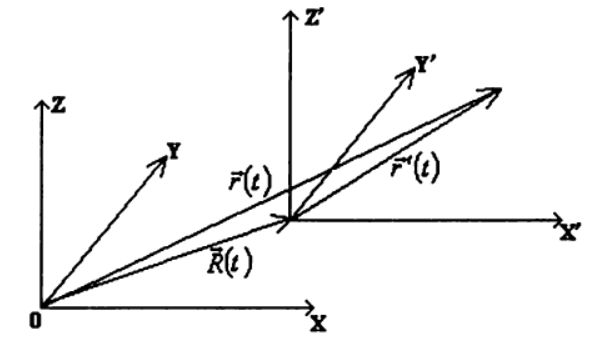
Thus, to find the law of motion of a point in an arbitrary reference system
it is necessary: 1) to set the law of motion of a point -
relative to the reference system ; 2) set the law of motion -
 reference systems relative to the reference system
 3) determine the law of motion of a point -
relative to the reference system .Construction of the Moon's orbit in the heliocentric reference system
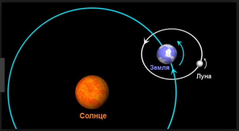
In the heliocentric reference system (system
) The earth moves in a circle of radius  km (period of circulation
  with.). The moon, in turn, moves around the Earth (system K ') in a circle of radius
 km (circulation period
 with. As is known [1,2], when a material point moves along a circle of radius
 with constant angular velocity
  The coordinates of the radius vector drawn from the origin to the current position of the point vary according to the law:
Where
 - the initial phase characterizing the position of the particle at the moment of time
  which we will assume to be zero later. Replacing in (3) on
  and
and  and substituting in (1), we obtain the dependence of the radius vector of the Moon in the heliocentric coordinate system on time:
Expression (4) sets the moon's orbit (
 ) in parametric form, where the parameter is time. To build the desired orbit by means of Python, we define the radii of the orbits and the periods of rotation of the Earth and the Moon.
 The earth moves in a heliocentric coordinate system (
) its orbit radius and orbital period are respectively equal  . The moon moves around the earth in the coordinate system () its orbit radius and orbital period are respectively equal
  .
. Taking into account (4), we define the functions of dependence of coordinates on time:

Using (5), we obtain a pair of coordinates for the moon's orbit:

Let us set the number of points where coordinates N = 1000 and discrete time are calculated on the interval of the period of rotation of the Earth
 . Let's write a program and build a graph for a positive coordinate change area:
Determination of the orbits of the Earth and the Moon
from numpy import*
from matplotlib.pyplot import*
R1=1.496*10**8#Числовые данные для расчётов взяты из  публикации [6]
T1=3.156*10**7
R2=3.844*10**5
T2=2.36*10**6
N=1000.0defX(t):return R1*cos(2*pi*t/T1)
defY(t):return R1*sin(2*pi*t/T1)
defx(t):return R2*cos(2*pi*t/T2)
defy(t):return R2*sin(2*pi*t/T2)
k=100
t=[T1*i/N for i in arange(0,k,1)]
X=array([X(w) for w in t])
Y=array([Y(w) for w in t])
x=array([x(w) for w in t])
y=array([y(w) for w in t])
XG=X+x
YG=Y+y
figure()
title("Траектория орбит Земли и Луны.\n Для положительных значений координат")
xlabel('$X(t_{k})$,$X_{g}(t_{k})$')
ylabel('$Y(t_{k})$,$Y_{g}(t_{k})$')
axis([1.2*10**8,1.5*10**8,0,1*10**8])
plot(X,Y,label='Орбита Земли')
plot(XG,YG,label='Орбита Луны')
legend(loc='best')
grid(True)
show()
We get:

Fig.1.
The created schedule allows you to expand the learning task and see what the moon's orbit will be if the moon's orbit radius is
 . . To the reader, even without special knowledge of astronomy, it is clear that the Moon cannot have such an orbit in the earth, not in the field of the Earth, but a hypothetical radius is used to study the conditions of the loops . Make the appropriate changes to the program:
Determination of the orbits of the Earth and the Moon
studying
from numpy import*
from matplotlib.pyplot import*
R1=1.496*10**8#Числовые данные для расчётов взяты из  публикации [6]
T1=3.156*10**7
R2=3.844*10**7
T2=2.36*10**6
N=1000.0defX(t):return R1*cos(2*pi*t/T1)
defY(t):return R1*sin(2*pi*t/T1)
defx(t):return R2*cos(2*pi*t/T2)
defy(t):return R2*sin(2*pi*t/T2)
t=[T1*i/N for i in arange(0,N,1)]
X=array([X(w) for w in t])
Y=array([Y(w) for w in t])
x=array([x(w) for w in t])
y=array([y(w) for w in t])
XG=X+x
YG=Y+y
figure()
title("Гелиоцентрическая орбита  Земли и Луны")
xlabel('$X(t_{k})$,$X_{g}(t_{k})$')
ylabel('$Y(t_{k})$,$Y_{g}(t_{k})$')
axis([-2.0*10**8,2.0*10**8,-2.0*10**8,2.0*10**8])
plot(X,Y,label='Орбита Земли')
plot(XG,YG,label='Орбита Луны')
legend(loc='best')
grid(True)
show()
We obtain:

Fig.2
Comparing the orbits of the Moon, presented in Fig. 1 and 2, we find their significant differences. To explain the reasons for these differences, it is necessary to compare the linear velocities of the Moon in the first and second cases and the linear velocity of the Earth.
Since the direction of the linear velocity of the Earth relative to the Sun, as well as the direction of the linear velocity of the Moon relative to the Earth, changes over time, and the speed remains constant in magnitude.
As a quantitative characteristic of the ratio of the linear velocities of the Moon and Earth in the heliocentric coordinate system, choose the difference between the module of the linear velocity of the Earth and the projection of the linear velocity of the Moon on the direction of the vector of the linear velocity of the Earth:

Define the functions that describe the laws of changes in the components of the velocity of the Earth and the Moon:

To determine the resulting speed, taking into account the projection, we use the relation:

We write the program taking into account (5), (8), (9) and the radius of the orbit of the moon
km:The moon and the earth are moving in the same direction
from numpy import*
from matplotlib.pyplot import*
R1=1.496*10**8#Числовые данные для расчётов взяты из  публикации [6]
T1=3.156*10**7
R2=3.844*10**5
T2=2.36*10**6
N=1000.0
k1=2*pi/T1
k2=2*pi/T2
defVx(t):return -k1*R1*sin(k1*t)
defVy(t):return k1*R1*cos(k1*t)
defvx(t):return -k2*R2*sin(k2*t)
defvy(t):return k2*R2*cos(k2*t)
defD(t):return sqrt(Vx(t)**2+Vy(t)**2)-sqrt(vx(t)**2+vy(t)**2)*(Vx(t)*vx(t)+Vy(t)*vy(t))/((sqrt(Vx(t)**2+Vy(t)**2))*(sqrt(vx(t)**2+vy(t)**2)))
x=[T1*i/N for i in arange(0,N,1)]
y=[D(t) for t in x]
title("Луна движется в  одном направлении с Землёй \n Радиус орбиты  Луны  R2=3.844*10**5 км.")
xlabel('t')
ylabel('D(t)')
plot(x,y)
show()
We get:

Fig.3.
Let's write the program taking into account (5), (8), (9) and the radius of the Moon's orbit R2 = 3.844 * 10 ** 7 km:
The moon periodically moves in the opposite direction to Earth.
from matplotlib.pyplot import*
R1=1.496*10**8#Числовые данные для расчётов взяты из  публикации [6]
T1=3.156*10**7
R2=3.844*10**7
T2=2.36*10**6
N=1000.0
k1=2*pi/T1
k2=2*pi/T2
defVx(t):return -k1*R1*sin(k1*t)
defVy(t):return k1*R1*cos(k1*t)
defvx(t):return -k2*R2*sin(k2*t)
defvy(t):return k2*R2*cos(k2*t)
defD(t):return sqrt(Vx(t)**2+Vy(t)**2)-sqrt(vx(t)**2+vy(t)**2)*(Vx(t)*vx(t)+Vy(t)*vy(t))/((sqrt(Vx(t)**2+Vy(t)**2))*(sqrt(vx(t)**2+vy(t)**2)))
x=[T1*i/N for i in arange(0,N,1)]
y=[D(t) for t in x]
title("  Периодически Луна движется в противоположном к Земле  \n направлению. Радиус орбиты  Луны  R2=3.844*10**7 км.")
xlabel('t')
ylabel('D(t)')
plot(x,y)
show()
We get:
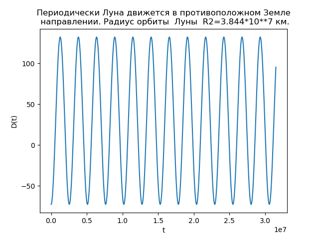
Fig.4.
Dependency analysis allows us to explain the reason for differences in orbits. D (t) function with
km is always positive, i.e. the moon always moves in the direction of the Earth’s motion and no loops form. With km magnitude  takes negative values, and there are times in which the moon moves in the opposite direction of the Earth’s motion, and therefore the orbit has loops. This was the meaning of the use in the calculations of the non-existent orbit of the moon.
The construction of the orbit of Mars in the reference system associated with the Earth
.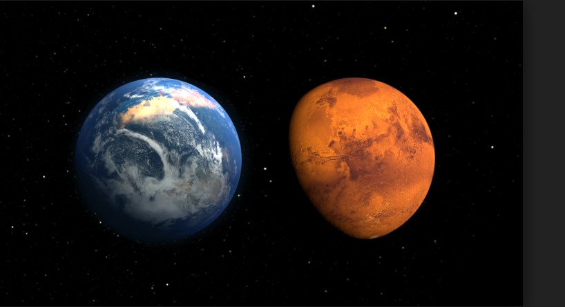
In the heliocentric reference system (system K), the Earth moves in a circle of radius
km, period of circulation  day, Mars moves along an ellipse, the semi-major axis of which
  km, the period of revolution of Mars
  day., eccentricity of the orbit
  [3]. The motion of the Earth is described by the radius vector R (t), given by expression (3). Due to the fact that the orbit of Mars is an ellipse, the dependencies
 from time are set parametrically [4]:
 , (ten)
 , (eleven)
 , (12) The
 total turnover by ellipse corresponds to a change in the parameter <img
 from 0 to
  . To build the Mars orbit, it is necessary to calculate at the same moments of time the coordinates of the radius vectors describing the position of the Earth and Mars in the heliocentric frame of reference, then in accordance with the relation
 calculate the coordinates of Mars in the reference system associated with the Earth.
 To build the orbit of Mars in the reference system associated with the Earth, we use the previously given parameters of the orbits of the Earth and Mars, relations (10) - (12), as well as relations for the coordinates of the Earth:
 , (13)
 , (14)
 It should be noted that the number of periods of Mars orbiting around the Sun is equal to
 , then the number of points at which the calculation should be made and the distance between them will be determined from the relations:
 (15)
(15)Mars orbit in the Earth's reference system
from numpy import*
from matplotlib.pyplot import*
R1=1.496*10e8#Числовые данные для расчётов взяты из  публикации [4]
T1=365.24
am=2.28*10e8
Tm=689.98
ee=0.093
N=36000defx(g):return am*(cos(g)-ee)
defy(g):return am*sqrt(1-ee**2)*sin(g)
deft(g):return Tm*(g-ee*sin(g))/2*pi
defX(g):return R1*cos(2*pi*t(g)/T1)
defY(g):return R1*sin(2*pi*t(g)/T1)
y=array([y(2*pi*i/N) for i in arange(0,N,1)])
x=array([x(2*pi*i/N) for i in arange(0,N,1)])
X=array([X(2*pi*i/N) for i in arange(0,N,1)])
Y=array([Y(2*pi*i/N) for i in arange(0,N,1)])
t=array([t(2*pi*i/N) for i in arange(0,N,1)])
figure()
title("Гелиоцентрические орбиты  Земли и Марса")
xlabel('x(g),X(g)')
ylabel('y(g),Y(g)')
plot(x,y,label='Орбита Марса')
plot(X,Y,label='Орбита Земли')
legend(loc='best')
figure()
title("Положение Марса в системе отсчёта связанной с Землёй")
xlabel('x1/10e8')
ylabel('y1(g/10e8')
x1=(x-X)
y1=(y-Y)
plot(x1/10e8,y1/10e8)
figure()
title("Зависимость расстояния между Землёй и Марсом \n от времени в годах")
xlabel('t/365.24')
ylabel('sqrt(x1**2+y1**2)/10e8')
y2=sqrt(x1**2+y1**2)/10e8
x2=t/365.24
plot(x2,y2)
show()
We obtain:
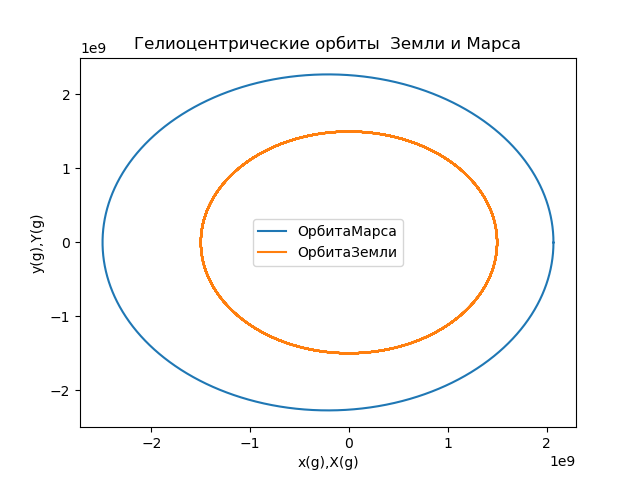
Fig.5
Calculate the coordinates of the radius vector describing the position of Mars in the reference system associated with the Earth, and build orbits (Fig.6) using the relation:
 (16)
(16) 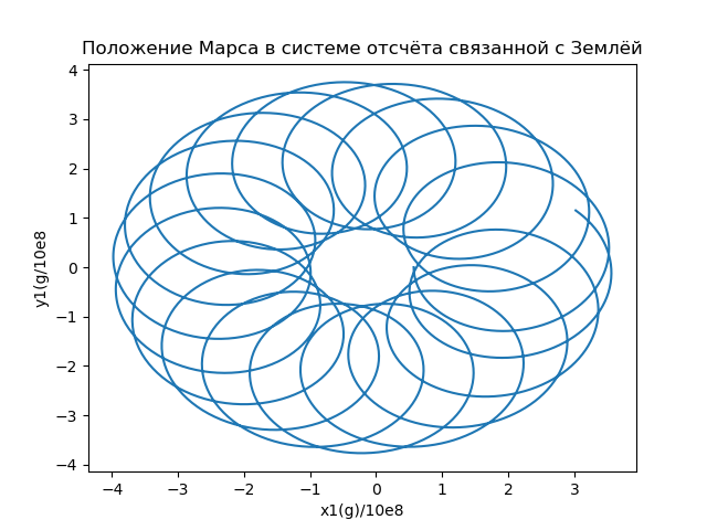
Fig.6
Another important characteristic of the motion of Mars (primarily for interplanetary space flights) is the distance between the Earth and Mars s (t), which is determined by the module of the radius vector describing the position of Mars in the reference system associated with the Earth. The dependence of the distance between the Earth and Mars on time, measured in Earth years, is shown in Fig.7.
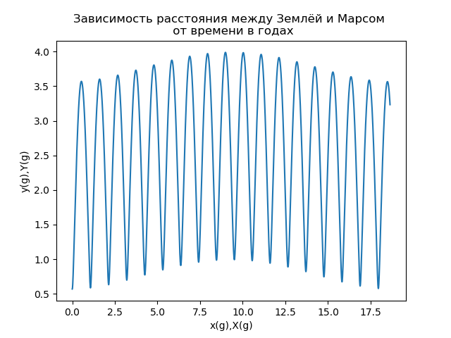
Pic.7
The analysis of the dependence presented in Fig. 7 shows that the distance between the Earth and Mars is a complex periodic function of time. If we use the terminology of the theory of signals [5], then we can say that the dependence s (t) is that it represents an amplitude-modulated signal, which is usually represented as a product of two functions of high-frequency (carrier) and low-frequency function, which specifies amplitude modulation (envelope) :
 (17)
(17) where
 - constant component of the function
  ;
;  - signal amplitude;
  - carrier frequency;
  - the amplitude of the function that specifies the depth of amplitude modulation;
 - frequency of the modulating function.
 It is seen from Fig. 7 that the carrier period is approximately 2 years, the period of the modulating function is approximately 17 years] 6].
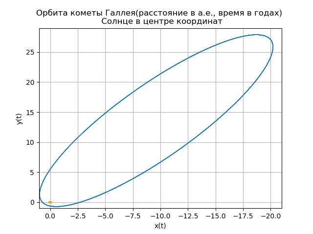
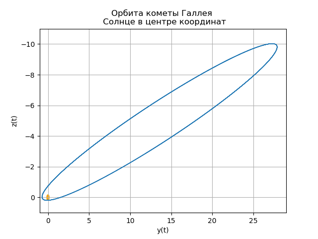
Constructing Heliocentric Orbit of Comet Halley
The last time Halley's comet passed through its perihelion (the point of the orbit closest to the Sun) was on February 9, 1986. (The Sun itself is considered to be located at the origin.) The
coordinates and velocity components of Halley’s comet were at that moment
 and
and  accordingly, the distance here is expressed in astronomical units of length - AU, or simply AU (an astronomical unit, i.e., the length of the major semi-major axis of the earth's orbit), and time — in years. In these units, the three-dimensional equations of motion of a comet are:
where:

Constructing Heliocentric Orbit of Comet Halley
from numpy import*
from scipy.integrate import odeint
import matplotlib.pyplot as plt
from matplotlib.patches import Circle
deff(y, t):
y1, y2, y3, y4,y5,y6 = y
return [y2, -(4*pi*pi*y1)/(y1**2+y3**2 +y5**2)**(3/2),y4,-(4*pi*pi*y3)/(y1**2+y3**2 +y5**2)**(3/2),y6,-(4*pi*pi*y5)/(y1**2+y3**2 +y5**2)**(3/2)]
t = linspace(0,300,10001)
y0 = [0.325514,-9.096111, -0.459460,-6.916686,0.166229,-1.305721]
[y1,y2, y3, y4,y5,y6]=odeint(f, y0, t, full_output=False).T
fig, ax = plt.subplots()
plt.title("Орбита кометы Галлея(расстояние в а.е., время в годах) \n Солнце в центре координат")
plt.xlabel('x(t)')
plt.ylabel('y(t)')
fig.set_facecolor('white')
ax.plot(y1,y3,linewidth=1)
circle = Circle((0, 0), 0.2, facecolor='orange')
ax.add_patch(circle)
plt.axis([1,-21,-1,29])
plt.grid(True)
fig, ax = plt.subplots()
plt.title("Орбита кометы Галлея \n Солнце в центре координат")
plt.xlabel('x(t)')
plt.ylabel('z(t)')
fig.set_facecolor('white')
ax.plot(y1,y5,linewidth=1)
circle = Circle((0, 0), 0.1, facecolor='orange')
ax.add_patch(circle)
plt.axis([1,-21,1,-11])
plt.grid(True)
fig, ax = plt.subplots()
plt.title("Орбита кометы Галлея \n Солнце в центре координат")
plt.xlabel('y(t)')
plt.ylabel('z(t)')
fig.set_facecolor('white')
ax.plot(y3,y5,linewidth=1)
circle = Circle((0, 0), 0.2, facecolor='orange')
ax.add_patch(circle)
plt.axis([-1,29,1,-11])
plt.grid(True)
fig, ax = plt.subplots()
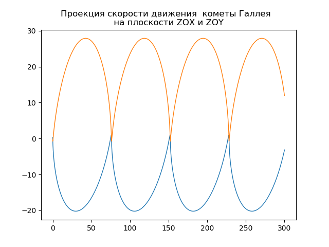
plt.title("Проекция скорости движения кометы Галлея \n на плоскости ZOX и ZOY ")
ax.plot(t,y1,linewidth=1)
ax.plot(t,y3,linewidth=1)
plt.show()Get:

Your own comet
Try an experiment. At night, you set up your telescope on top, not far from your home elevation. The night should be clear, cloudless, stellar, and if fortune smiled at you: at 0.30 am you will notice a new comet.
After repeated observations on the following nights, you will be able to calculate its coordinates on that first night. Coordinates in the heliocentric coordinate system: P0 = (x0, y0, z0) and the velocity vector v0 = (vx0, vy0, vz0).
Using this data, determine:
- distance of the comet from the Sun at perihelion (the closest point of the orbit to the Sun) and aphelion (the farthest point of the orbit from the Sun);
- the speed of the comet during its passage through perihelion and through aphelion;
- the period of circulation of the comet around the sun;
- The following two dates of passage of the comet through perihelion.
If you measure the distance in astronomical units, and time - in years, then the equation of motion of the comet will take the form (18). For your own comet, choose arbitrary starting coordinates and velocities of the same order as that of comet Halley.
If necessary, re-perform an arbitrary choice of the initial position and velocity vector until you get a plausible eccentric orbit that goes beyond the limits of the Earth's orbit (like most true comets).
References:
- Feynman R., Leighton R., Sands M. The Feynman Lectures on Physics. 3rd ed. T. 1.-2. M .: Mir, 1977.
- Matveev A. N. Mechanics and Theory of Relativity. M .: Higher. shk., 1986.
- Physical Encyclopedia. T. 3. M .: Great Russian Encyclopedia, 1992.
- Landau, LD, Lifshits, EM. A Course in Theoretical Physics. Mechanics. M .: Fyut-Matgiz, 1958.
- Baskakov S.I. Radio engineering circuits and signals. M .: Higher. shk., 1988.
- Porshnev C.V. Computer simulation of physical processes using the mathcad package .