Kalman Filter - Introduction
The Kalman filter is probably the most popular filtering algorithm used in many fields of science and technology. Due to its simplicity and effectiveness, it can be found in GPS-receivers, processors of sensor readings, when implementing control systems, etc.
There are a lot of articles and books about the Kalman filter on the Internet (mainly in English), but these articles have a rather high threshold for entry, there are many vague places, although in fact this is a very clear and transparent algorithm. I will try to talk about him in simple language, with a gradual increase in complexity.
Any measuring device has some error, a large number of external and internal influences can affect it, which leads to the fact that the information from it is noisy. The more noisy the data, the more difficult it is to process such information.
A filter is a data processing algorithm that removes noise and excess information. In the Kalman filter, it is possible to set a priori information about the nature of the system, the relationship of variables and based on this to build a more accurate estimate, but even in the simplest case (without entering a priori information) it gives excellent results.
Consider the simplest example - suppose we need to control the fuel level in the tank. To do this, a capacitive sensor is installed in the tank, it is very easy to maintain, but has some drawbacks - for example, dependence on refueling (the dielectric constant of the fuel depends on many factors, for example, temperature), the big influence of the “chatter” in the tank. As a result, the information from it represents a typical "saw" with a decent amplitude. Such sensors are often installed on heavy mining equipment (do not be confused by the volume of the tank):
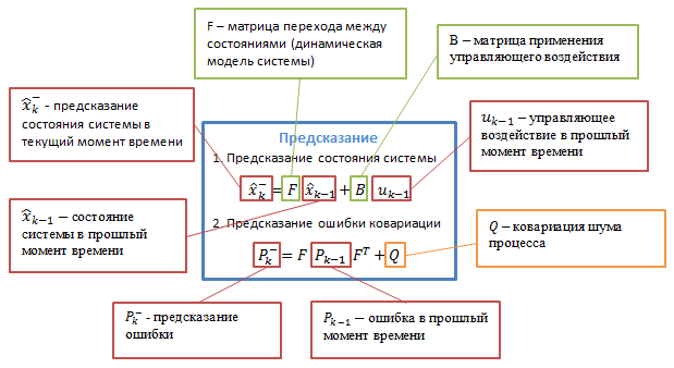
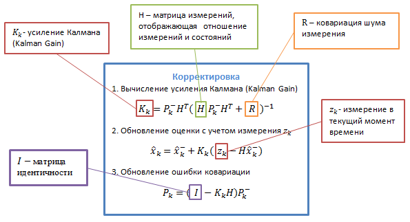
Let's digress a bit and get acquainted with the algorithm itself. The Kalman filter uses a dynamic model of the system (for example, the physical law of motion), well-known control actions and many sequential measurements to form the optimal state estimate. The algorithm consists of two repeating phases: prediction and adjustment. At the first, the prediction of the state at the next moment in time is calculated (taking into account the inaccuracy of their measurement). On the second, the new information from the sensor corrects the predicted value (also taking into account the inaccuracy and noisiness of this information):

The equations are presented in matrix form, if you do not know linear algebra - it's okay, then there will be a simplified version without matrices for the case with one variable. In the case of a single variable, matrices degenerate into scalar values.
Let’s take a look at the notation first: the subscript indicates the point in time: k is the current, (k-1) is the previous one, the minus sign in the upper index indicates that this is a predicted intermediate value.
The description of the variables is presented in the following images:
It is possible to describe for a long time and tediously what all these mysterious transition matrices mean, but it is better, in my opinion, to try using an algorithm using a real example - so that the abstract values find real meaning.
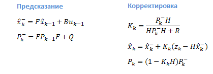
Let us return to the example with the fuel level sensor, since the state of the system is represented by one variable (fuel volume in the tank), the matrices degenerate into the usual equations:
In order to apply a filter, it is necessary to determine the matrices / values of the variables that determine the dynamics of the system and the measurements F, B and H:
F is a variable that describes the dynamics of the system, in the case of fuel, it can be a coefficient determining the fuel consumption at idle during the sampling time ( time between steps of the algorithm). However, in addition to fuel consumption, there are also gas stations ... therefore, for simplicity, we take this variable equal to 1 (that is, we indicate that the predicted value will be equal to the previous state).
B- a variable that determines the application of control action. If we had additional information about the engine speed or the degree of depressing the accelerator pedal, this parameter would determine how the fuel consumption will change during sampling. Since there are no control actions in our model (there is no information about them), we take B = 0.
H is the matrix that determines the relationship between measurements and the state of the system, until without explanation we take this variable also equal to 1.
R - measurement error can be determined by testing measuring instruments and determining the error of their measurement.
Q - determination of process noise is a more difficult task, since it is necessary to determine the variance of the process, which is not always possible. In any case, this parameter can be selected to provide the required level of filtration.
To dispel the remaining obscurity, we implement a simplified algorithm in C # (without matrices and control action):
The result of filtering with these parameters is shown in the figure (to adjust the degree of smoothing - you can change the Q and R parameters):
The most interesting thing remained outside the scope of the article - the Kalman filter for several variables, setting the relationship between them and automatically displaying values for unobserved variables. I will try to continue the topic as soon as the time appears.
I hope the description doesn’t turn out to be very tiring and complicated, if you still have questions and clarifications - welcome to comments)
UPD: List of sources:
CS373 - PROGRAMMING A ROBOTIC CAR - I highly recommend
Wikipedia (Russian)
Wikipedia (English)
On the hub: 1 and 2
More serious sources:
Greg Welch, Gary Bishop, “An Introduction to the Kalman Filter”, 2001
MSGrewal, AP Andrews, “Kalman Filtering - Theory and Practice Using MATLAB”, Wiley, 2001
UPD2: the example in this article is a purely demo one. The main application of the filter is more complex systems. For example, in the case of determining the coordinates of a car, you can relate the GPS coordinates, steering angle, engine speed ... and all this will increase the accuracy of coordinates.
There are a lot of articles and books about the Kalman filter on the Internet (mainly in English), but these articles have a rather high threshold for entry, there are many vague places, although in fact this is a very clear and transparent algorithm. I will try to talk about him in simple language, with a gradual increase in complexity.
What is it for?
Any measuring device has some error, a large number of external and internal influences can affect it, which leads to the fact that the information from it is noisy. The more noisy the data, the more difficult it is to process such information.
A filter is a data processing algorithm that removes noise and excess information. In the Kalman filter, it is possible to set a priori information about the nature of the system, the relationship of variables and based on this to build a more accurate estimate, but even in the simplest case (without entering a priori information) it gives excellent results.
Consider the simplest example - suppose we need to control the fuel level in the tank. To do this, a capacitive sensor is installed in the tank, it is very easy to maintain, but has some drawbacks - for example, dependence on refueling (the dielectric constant of the fuel depends on many factors, for example, temperature), the big influence of the “chatter” in the tank. As a result, the information from it represents a typical "saw" with a decent amplitude. Such sensors are often installed on heavy mining equipment (do not be confused by the volume of the tank):
Kalman Filter
Let's digress a bit and get acquainted with the algorithm itself. The Kalman filter uses a dynamic model of the system (for example, the physical law of motion), well-known control actions and many sequential measurements to form the optimal state estimate. The algorithm consists of two repeating phases: prediction and adjustment. At the first, the prediction of the state at the next moment in time is calculated (taking into account the inaccuracy of their measurement). On the second, the new information from the sensor corrects the predicted value (also taking into account the inaccuracy and noisiness of this information):
The equations are presented in matrix form, if you do not know linear algebra - it's okay, then there will be a simplified version without matrices for the case with one variable. In the case of a single variable, matrices degenerate into scalar values.
Let’s take a look at the notation first: the subscript indicates the point in time: k is the current, (k-1) is the previous one, the minus sign in the upper index indicates that this is a predicted intermediate value.
The description of the variables is presented in the following images:
It is possible to describe for a long time and tediously what all these mysterious transition matrices mean, but it is better, in my opinion, to try using an algorithm using a real example - so that the abstract values find real meaning.
We will test in
Let us return to the example with the fuel level sensor, since the state of the system is represented by one variable (fuel volume in the tank), the matrices degenerate into the usual equations:
Process Model Definition
In order to apply a filter, it is necessary to determine the matrices / values of the variables that determine the dynamics of the system and the measurements F, B and H:
F is a variable that describes the dynamics of the system, in the case of fuel, it can be a coefficient determining the fuel consumption at idle during the sampling time ( time between steps of the algorithm). However, in addition to fuel consumption, there are also gas stations ... therefore, for simplicity, we take this variable equal to 1 (that is, we indicate that the predicted value will be equal to the previous state).
B- a variable that determines the application of control action. If we had additional information about the engine speed or the degree of depressing the accelerator pedal, this parameter would determine how the fuel consumption will change during sampling. Since there are no control actions in our model (there is no information about them), we take B = 0.
H is the matrix that determines the relationship between measurements and the state of the system, until without explanation we take this variable also equal to 1.
Determination of smoothing properties
R - measurement error can be determined by testing measuring instruments and determining the error of their measurement.
Q - determination of process noise is a more difficult task, since it is necessary to determine the variance of the process, which is not always possible. In any case, this parameter can be selected to provide the required level of filtration.
We implement in code
To dispel the remaining obscurity, we implement a simplified algorithm in C # (without matrices and control action):
class KalmanFilterSimple1D
{
public double X0 {get; private set;} // predicted state
public double P0 { get; private set; } // predicted covariance
public double F { get; private set; } // factor of real value to previous real value
public double Q { get; private set; } // measurement noise
public double H { get; private set; } // factor of measured value to real value
public double R { get; private set; } // environment noise
public double State { get; private set; }
public double Covariance { get; private set; }
public KalmanFilterSimple1D(double q, double r, double f = 1, double h = 1)
{
Q = q;
R = r;
F = f;
H = h;
}
public void SetState(double state, double covariance)
{
State = state;
Covariance = covariance;
}
public void Correct(double data)
{
//time update - prediction
X0 = F*State;
P0 = F*Covariance*F + Q;
//measurement update - correction
var K = H*P0/(H*P0*H + R);
State = X0 + K*(data - H*X0);
Covariance = (1 - K*H)*P0;
}
}
// Применение...
var fuelData = GetData();
var filtered = new List();
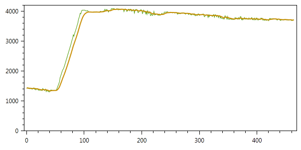
var kalman = new KalmanFilterSimple1D(f: 1, h: 1, q: 2, r: 15); // задаем F, H, Q и R
kalman.SetState(fuelData[0], 0.1); // Задаем начальные значение State и Covariance
foreach(var d in fuelData)
{
kalman.Correct(d); // Применяем алгоритм
filtered.Add(kalman.State); // Сохраняем текущее состояние
}
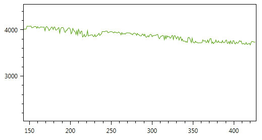
The result of filtering with these parameters is shown in the figure (to adjust the degree of smoothing - you can change the Q and R parameters):
The most interesting thing remained outside the scope of the article - the Kalman filter for several variables, setting the relationship between them and automatically displaying values for unobserved variables. I will try to continue the topic as soon as the time appears.
I hope the description doesn’t turn out to be very tiring and complicated, if you still have questions and clarifications - welcome to comments)
UPD: List of sources:
CS373 - PROGRAMMING A ROBOTIC CAR - I highly recommend
Wikipedia (Russian)
Wikipedia (English)
On the hub: 1 and 2
More serious sources:
Greg Welch, Gary Bishop, “An Introduction to the Kalman Filter”, 2001
MSGrewal, AP Andrews, “Kalman Filtering - Theory and Practice Using MATLAB”, Wiley, 2001
UPD2: the example in this article is a purely demo one. The main application of the filter is more complex systems. For example, in the case of determining the coordinates of a car, you can relate the GPS coordinates, steering angle, engine speed ... and all this will increase the accuracy of coordinates.