Overview of Data Clustering Algorithms
Greetings!
In my thesis, I conducted a review and comparative analysis of data clustering algorithms. I thought that already collected and worked out material may be interesting and useful to someone.
What clustering is, sashaeve said in the article “Clustering: k-means and c-means algorithms” . I will partially repeat the words of Alexander, partially supplement. Also at the end of this article, those interested can read the materials from the links in the list of references.
I also tried to bring the dry "diploma" style of presentation to a more journalistic one.
Clustering (or cluster analysis) is the task of breaking down multiple objects into groups called clusters. Inside each group there should be “similar” objects, and objects of different groups should be as different as possible. The main difference between clustering and classification is that the list of groups is not clearly defined and is determined during the operation of the algorithm.
The application of cluster analysis in general is reduced to the following steps:
After receiving and analyzing the results, it is possible to adjust the selected metric and clustering method to obtain the optimal result.
So, how to determine the "similarity" of objects? First you need to create a vector of characteristics for each object - as a rule, this is a set of numerical values, for example, a person’s height-weight. However, there are also algorithms that work with qualitative (so-called categorical) characteristics.
After we have determined the vector of characteristics, we can normalize so that all components make the same contribution in calculating the “distance”. In the normalization process, all values are reduced to a certain range, for example, [-1, -1] or [0, 1].
Finally, for each pair of objects, the "distance" between them is measured - the degree of similarity. There are many metrics, here are just the main ones:
The choice of metric lies entirely with the researcher, since the results of clustering can differ significantly when using different measures.
For myself, I have identified two main classifications of clustering algorithms.
In the case of hierarchical algorithms, the question arises of how to combine clusters, how to calculate the "distance" between them. There are several metrics:
Among the hierarchical clustering algorithms, two main types are distinguished: upstream and downstream algorithms. Top-down algorithms work according to the “top-down” principle: at the beginning, all objects are placed in one cluster, which is then divided into ever smaller clusters. Upstream algorithms are more common, which at the beginning of work put each object in a separate cluster, and then combine the clusters into larger and larger ones until all the objects in the selection are contained in one cluster. Thus, a system of nested partitions is constructed. The results of such algorithms are usually presented in the form of a tree - dendrograms. A classic example of such a tree is the classification of animals and plants.
To calculate the distances between clusters, more often than not everyone uses two distances: a single link or a full link (see the overview of measures of distances between clusters).
The disadvantage of hierarchical algorithms is the system of complete partitions, which may be redundant in the context of the problem being solved.
The task of clustering can be considered as building the optimal partition of objects into groups. Moreover, optimality can be defined as the requirement to minimize the mean square error of the partition:
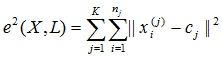
where c j is the “center of mass” of the cluster j (the point with the average values of the characteristics for this cluster).
Quadratic error algorithms are a type of flat algorithm. The most common algorithm in this category is the k-means method. This algorithm builds a given number of clusters located as far as possible from each other. The algorithm is divided into several stages:
As a criterion for stopping the operation of the algorithm, the minimum change in the standard error is usually chosen. It is also possible to stop the operation of the algorithm if, in step 2, there were no objects moving from the cluster to the cluster.
The disadvantages of this algorithm include the need to specify the number of clusters for the partition.
The most popular fuzzy clustering algorithm is the c-means algorithm. It is a modification of the k-means method. The steps of the algorithm:
This algorithm may not be suitable if the number of clusters is not known in advance, or it is necessary to unambiguously assign each object to one cluster.
The essence of such algorithms is that the sample of objects is represented in the form of a graph G = (V, E) , the vertices of which correspond to objects, and the edges have a weight equal to the "distance" between the objects. The advantages of graph clustering algorithms are visibility, relative ease of implementation and the possibility of making various improvements based on geometric considerations. The main algorithms are the algorithm for selecting connected components, the algorithm for constructing the minimum spanning tree, and the layer-by-layer clustering algorithm.
In the algorithm for selecting connected components, the input parameter R is set and in the graph all edges for which the "distances" are greater than R are deleted . Only the closest pairs of objects remain connected. The meaning of the algorithm is to select such a value of R that lies in the range of all “distances” at which the graph “falls apart” into several connected components. The resulting components are clusters.
To select the parameter R , a histogram of the distributions of pairwise distances is usually constructed. In problems with a well-defined cluster data structure, the histogram will have two peaks - one corresponds to intracluster distances, the second to intercluster distances. R parameterselected from the minimum zone between these peaks. At the same time, it is rather difficult to control the number of clusters using the distance threshold.
The minimum spanning tree algorithm first builds a minimal spanning tree on the graph, and then sequentially removes the edges with the highest weight. The figure shows the minimum spanning tree obtained for nine objects.
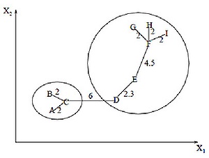
By removing the bond labeled CD with a length of 6 units (edge with maximum distance), we obtain two clusters: {A, B, C} and {D, E, F, G, H, I}. The second cluster can be further divided into two more clusters by removing the edge EF, which has a length equal to 4.5 units.
The layer-by-layer clustering algorithm is based on the selection of connected components of the graph at a certain level of distances between objects (vertices). The distance level is set by the distance threshold c . For example, if the distance between objects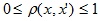 , then
  .
.
Algorithm layered clustering generates a sequence of subgraphs of G , which represent hierarchical relations between clusters
 ,
,
where G t = (V, E t ) - graph at level with t ,
 ,
,
with t - t-th threshold distance,
m - the number of hierarchical levels,
G 0 = (V, o), o is the empty set of edges of the graph obtained at t 0 = 1,
G m = G , that is, the graph of objects without restrictions on the distance (the length of the edges of the graph), since t m = 1.
By changing the distance thresholds { c 0 , ..., with m }, where 0 = с 0 < с 1 <... < с m = 1, it is possible to control the depth of the hierarchy of the resulting clusters. Thus, the layer-by-layer clustering algorithm is capable of creating both a flat data partition and a hierarchical one.
Computational Complexity of Algorithms
Algorithm Comparison Chart
In my work, I needed to select separate areas from hierarchical structures (trees). Those. essentially it was necessary to cut the original tree into several smaller trees. Since the oriented tree is a special case of a graph, algorithms based on graph theory are naturally suitable.
Unlike a fully connected graph, not all vertices are connected by edges in an oriented tree, while the total number of edges is n – 1, where n is the number of vertices. Those. in relation to the nodes of the tree, the operation of the algorithm for selecting connected components will be simplified, since removing any number of edges will “break up” the tree into connected components (individual trees). The minimal spanning tree algorithm in this case will coincide with the algorithm for selecting connected components - by removing the longest edges, the original tree is split into several trees. It is obvious that the construction phase of the smallest spanning tree is skipped.
In the case of using other algorithms, they would have to separately take into account the presence of relations between objects, which complicates the algorithm.
Separately, I want to say that in order to achieve the best result, it is necessary to experiment with the choice of distance measures, and sometimes even change the algorithm. There is no single solution.
1. Vorontsov K.V. Clustering and multidimensional scaling algorithms . Lecture course. Moscow State University, 2007.
2. Jain A., Murty M., Flynn P. Data Clustering: A Review . // ACM Computing Surveys. 1999. Vol. 31, no. 3.
3. Kotov A., Krasilnikov N. Data clustering . 2006.
3. Mandel I. D. Cluster analysis. - M .: Finance and Statistics, 1988.
4. Applied statistics: classification and reduction of dimension. / S.A. Ayvazyan, V.M. Buchstaber, I.S. Enyukov, L.D. Meshalkin - M .: Finance and Statistics, 1989.
5. Information and analytical resource on machine learning, pattern recognition and data mining - www.machinelearning.ru
6. Chubukova I.A. Lecture course “Data Mining”, Internet University of Information Technologies - www.intuit.ru/department/database/datamining
In my thesis, I conducted a review and comparative analysis of data clustering algorithms. I thought that already collected and worked out material may be interesting and useful to someone.
What clustering is, sashaeve said in the article “Clustering: k-means and c-means algorithms” . I will partially repeat the words of Alexander, partially supplement. Also at the end of this article, those interested can read the materials from the links in the list of references.
I also tried to bring the dry "diploma" style of presentation to a more journalistic one.
The concept of clustering
Clustering (or cluster analysis) is the task of breaking down multiple objects into groups called clusters. Inside each group there should be “similar” objects, and objects of different groups should be as different as possible. The main difference between clustering and classification is that the list of groups is not clearly defined and is determined during the operation of the algorithm.
The application of cluster analysis in general is reduced to the following steps:
- Selecting a selection of objects for clustering.
- Definition of a set of variables by which objects in the sample will be evaluated. If necessary, normalize the values of variables.
- Calculation of values of a measure of similarity between objects.
- Application of the cluster analysis method to create groups of similar objects (clusters).
- Presentation of analysis results.
After receiving and analyzing the results, it is possible to adjust the selected metric and clustering method to obtain the optimal result.
Distance measures
So, how to determine the "similarity" of objects? First you need to create a vector of characteristics for each object - as a rule, this is a set of numerical values, for example, a person’s height-weight. However, there are also algorithms that work with qualitative (so-called categorical) characteristics.
After we have determined the vector of characteristics, we can normalize so that all components make the same contribution in calculating the “distance”. In the normalization process, all values are reduced to a certain range, for example, [-1, -1] or [0, 1].
Finally, for each pair of objects, the "distance" between them is measured - the degree of similarity. There are many metrics, here are just the main ones:
- Euclidean distance
The most common distance function. Represents a geometric distance in multidimensional space: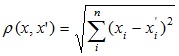
- Squared Euclidean distance
Used to give more weight to objects that are more distant from each other. This distance is calculated as follows:
- City Quarter Distance (Manhattan distance)
This distance is the average of the differences in coordinates. In most cases, this measure of distance leads to the same results as for the usual Euclidean distance. However, for this measure, the influence of individual large differences (emissions) is reduced (since they are not squared). Formula for calculating the Manhattan distance:
- Chebyshev
distance This distance can be useful when you need to define two objects as “different” if they differ in any one coordinate. The Chebyshev distance is calculated by the formula:
- Power distance
Applies when it is necessary to increase or decrease the weight related to the dimension for which the corresponding objects are very different. Power of the distance calculated by the following formula ,
,
where r and p - the parameters defined by the user. The parameter p is responsible for the gradual weighting of differences by individual coordinates, the parameter r is responsible for the progressive weighing of large distances between objects. If both parameters - r and p - are equal to two, then this distance coincides with the Euclidean distance.
The choice of metric lies entirely with the researcher, since the results of clustering can differ significantly when using different measures.
Algorithm Classification
For myself, I have identified two main classifications of clustering algorithms.
- Hierarchical and flat.
Hierarchical algorithms (also called taxonomy algorithms) build not just one partition of the sample into disjoint clusters, but a system of nested partitions. T.O. at the output, we get a tree of clusters, the root of which is the entire sample, and the leaves are the smallest clusters.
Flat algorithms build one partition of objects into clusters. - Clear and fuzzy.
Clear (or disjoint) algorithms associate a cluster number with each sample object, i.e. each object belongs to only one cluster. Fuzzy (or intersecting) algorithms for each object associate a set of real values that show the degree of the relationship of the object to the clusters. Those. each object belongs to each cluster with some probability.
Clustering
In the case of hierarchical algorithms, the question arises of how to combine clusters, how to calculate the "distance" between them. There are several metrics:
- Single communication (distance of the nearest neighbor)
In this method, the distance between two clusters is determined by the distance between the two closest objects (nearest neighbors) in different clusters. The resulting clusters tend to chain together. - Full communication (distance of the most distant neighbors)
In this method, the distances between the clusters are determined by the largest distance between any two objects in different clusters (i.e., the most distant neighbors). This method usually works very well when objects come from separate groups. If the clusters are elongated or their natural type is "chain", then this method is unsuitable. - Unweighted pairwise mean
In this method, the distance between two different clusters is calculated as the average distance between all pairs of objects in them. The method is effective when objects form different groups, but it works equally well in cases of extended ("chain" type) clusters. - Weighted pairwise average
The method is identical to the method of unweighted pairwise average, except that in calculations the size of the corresponding clusters (i.e. the number of objects contained in them) is used as a weight coefficient. Therefore, this method should be used when unequal cluster sizes are assumed. - Unweighted Centroid Method
In this method, the distance between two clusters is defined as the distance between their centers of gravity. - Weighted Centroid Method (Median)
This method is identical to the previous one, except that the calculations use weights to account for the difference between cluster sizes. Therefore, if there are or are suspected of significant differences in cluster sizes, this method is preferable to the previous one.
Algorithm Overview
Hierarchical Clustering Algorithms
Among the hierarchical clustering algorithms, two main types are distinguished: upstream and downstream algorithms. Top-down algorithms work according to the “top-down” principle: at the beginning, all objects are placed in one cluster, which is then divided into ever smaller clusters. Upstream algorithms are more common, which at the beginning of work put each object in a separate cluster, and then combine the clusters into larger and larger ones until all the objects in the selection are contained in one cluster. Thus, a system of nested partitions is constructed. The results of such algorithms are usually presented in the form of a tree - dendrograms. A classic example of such a tree is the classification of animals and plants.
To calculate the distances between clusters, more often than not everyone uses two distances: a single link or a full link (see the overview of measures of distances between clusters).
The disadvantage of hierarchical algorithms is the system of complete partitions, which may be redundant in the context of the problem being solved.
Quadratic Error Algorithms
The task of clustering can be considered as building the optimal partition of objects into groups. Moreover, optimality can be defined as the requirement to minimize the mean square error of the partition:
where c j is the “center of mass” of the cluster j (the point with the average values of the characteristics for this cluster).
Quadratic error algorithms are a type of flat algorithm. The most common algorithm in this category is the k-means method. This algorithm builds a given number of clusters located as far as possible from each other. The algorithm is divided into several stages:
- Randomly select k points that are the initial "centers of mass" of the clusters.
- Assign each object to a cluster with the nearest “center of mass”.
- Recalculate the "centers of mass" of the clusters according to their current composition.
- If the criterion for stopping the algorithm is not satisfied, return to step 2.
As a criterion for stopping the operation of the algorithm, the minimum change in the standard error is usually chosen. It is also possible to stop the operation of the algorithm if, in step 2, there were no objects moving from the cluster to the cluster.
The disadvantages of this algorithm include the need to specify the number of clusters for the partition.
Fuzzy algorithms
The most popular fuzzy clustering algorithm is the c-means algorithm. It is a modification of the k-means method. The steps of the algorithm:
- Select the initial fuzzy partition of n objects into k clusters by choosing the membership matrix U of size nxk .
- Using the U matrix, find the value of fuzzy error criterion:
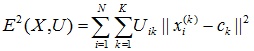 ,
,
where c the k - «center of mass" of the fuzzy cluster the k : .
. - Regroup objects in order to reduce this value of the fuzzy error criterion.
- Return to step 2 until the changes in the matrix U become insignificant.
This algorithm may not be suitable if the number of clusters is not known in advance, or it is necessary to unambiguously assign each object to one cluster.
Graph Based Algorithms
The essence of such algorithms is that the sample of objects is represented in the form of a graph G = (V, E) , the vertices of which correspond to objects, and the edges have a weight equal to the "distance" between the objects. The advantages of graph clustering algorithms are visibility, relative ease of implementation and the possibility of making various improvements based on geometric considerations. The main algorithms are the algorithm for selecting connected components, the algorithm for constructing the minimum spanning tree, and the layer-by-layer clustering algorithm.
Connected Component Algorithm
In the algorithm for selecting connected components, the input parameter R is set and in the graph all edges for which the "distances" are greater than R are deleted . Only the closest pairs of objects remain connected. The meaning of the algorithm is to select such a value of R that lies in the range of all “distances” at which the graph “falls apart” into several connected components. The resulting components are clusters.
To select the parameter R , a histogram of the distributions of pairwise distances is usually constructed. In problems with a well-defined cluster data structure, the histogram will have two peaks - one corresponds to intracluster distances, the second to intercluster distances. R parameterselected from the minimum zone between these peaks. At the same time, it is rather difficult to control the number of clusters using the distance threshold.
Minimum Spanning Tree Algorithm
The minimum spanning tree algorithm first builds a minimal spanning tree on the graph, and then sequentially removes the edges with the highest weight. The figure shows the minimum spanning tree obtained for nine objects.
By removing the bond labeled CD with a length of 6 units (edge with maximum distance), we obtain two clusters: {A, B, C} and {D, E, F, G, H, I}. The second cluster can be further divided into two more clusters by removing the edge EF, which has a length equal to 4.5 units.
Layer-by-layer clustering
The layer-by-layer clustering algorithm is based on the selection of connected components of the graph at a certain level of distances between objects (vertices). The distance level is set by the distance threshold c . For example, if the distance between objects
, then . Algorithm layered clustering generates a sequence of subgraphs of G , which represent hierarchical relations between clusters
, where G t = (V, E t ) - graph at level with t ,
, with t - t-th threshold distance,
m - the number of hierarchical levels,
G 0 = (V, o), o is the empty set of edges of the graph obtained at t 0 = 1,
G m = G , that is, the graph of objects without restrictions on the distance (the length of the edges of the graph), since t m = 1.
By changing the distance thresholds { c 0 , ..., with m }, where 0 = с 0 < с 1 <... < с m = 1, it is possible to control the depth of the hierarchy of the resulting clusters. Thus, the layer-by-layer clustering algorithm is capable of creating both a flat data partition and a hierarchical one.
Algorithm Comparison
Computational Complexity of Algorithms
| Clustering algorithm | Computational complexity |
| Hierarchical | O (n 2 ) |
| k-means | O (nkl), where k is the number of clusters, l is the number of iterations |
|---|---|
| c-medium | |
| Selection of connected components | depends on the algorithm |
| Minimum spanning tree | O (n 2 log n) |
| Layer-by-layer clustering | O (max (n, m)), where m <n (n-1) / 2 |
Algorithm Comparison Chart
| Clustering algorithm | Cluster shape | Input data | results |
| Hierarchical | Arbitrary | The number of clusters or distance threshold for truncating a hierarchy | Binary Cluster Tree |
| k-means | Hypersphere | Number of clusters | Cluster Centers |
| c-medium | Hypersphere | The number of clusters, the degree of fuzziness | Cluster centers, membership matrix |
| Selection of connected components | Arbitrary | Distance threshold R | Tree structure of clusters |
| Minimum spanning tree | Arbitrary | Number of clusters or distance threshold for edge removal | Tree structure of clusters |
| Layer-by-layer clustering | Arbitrary | Distance threshold sequence | Tree structure of clusters with different levels of hierarchy |
A bit about application
In my work, I needed to select separate areas from hierarchical structures (trees). Those. essentially it was necessary to cut the original tree into several smaller trees. Since the oriented tree is a special case of a graph, algorithms based on graph theory are naturally suitable.
Unlike a fully connected graph, not all vertices are connected by edges in an oriented tree, while the total number of edges is n – 1, where n is the number of vertices. Those. in relation to the nodes of the tree, the operation of the algorithm for selecting connected components will be simplified, since removing any number of edges will “break up” the tree into connected components (individual trees). The minimal spanning tree algorithm in this case will coincide with the algorithm for selecting connected components - by removing the longest edges, the original tree is split into several trees. It is obvious that the construction phase of the smallest spanning tree is skipped.
In the case of using other algorithms, they would have to separately take into account the presence of relations between objects, which complicates the algorithm.
Separately, I want to say that in order to achieve the best result, it is necessary to experiment with the choice of distance measures, and sometimes even change the algorithm. There is no single solution.
List of references
1. Vorontsov K.V. Clustering and multidimensional scaling algorithms . Lecture course. Moscow State University, 2007.
2. Jain A., Murty M., Flynn P. Data Clustering: A Review . // ACM Computing Surveys. 1999. Vol. 31, no. 3.
3. Kotov A., Krasilnikov N. Data clustering . 2006.
3. Mandel I. D. Cluster analysis. - M .: Finance and Statistics, 1988.
4. Applied statistics: classification and reduction of dimension. / S.A. Ayvazyan, V.M. Buchstaber, I.S. Enyukov, L.D. Meshalkin - M .: Finance and Statistics, 1989.
5. Information and analytical resource on machine learning, pattern recognition and data mining - www.machinelearning.ru
6. Chubukova I.A. Lecture course “Data Mining”, Internet University of Information Technologies - www.intuit.ru/department/database/datamining