B-tree data structure
- Transfer
Hello! We launched a new set for the course "Algorithms for Developers" and today we want to share an interesting translation prepared for students of this course.

In search trees, such as binary search tree, AVL tree, red-black tree, etc. each node contains only one value (key) and a maximum of two descendants. However, there is a special type of search tree called the B-tree (pronounced Bi-tree). In it, the node contains more than one value (key) and more than two descendants. The B-tree was developed in 1972 by Bayer and McCrate and was called the Height Balanced m-way Search Tree . Its modern name B-tree received later.
A B-tree can be defined as follows:
A B-tree is a balanced search tree in which each node contains many keys and has more than two children.
Here, the number of keys in the node and the number of its descendants depends on the order of the B-tree. Each B-tree has an order.
A B-tree of order m has the following properties:
Property 1: The depth of all leaves is the same.
Property 2: All nodes except the root must have at least (m / 2) - 1 keys and a maximum of m-1 keys.
Property 3: All nodes without leaves, except the root (i.e., all internal nodes), must have a minimum of m / 2 descendants.
Property 4:If the root is a leafless node, it must have at least 2 descendants.
Property 5: A node without leaves with n-1 keys must have n children.
Property 6: All keys in the node should be arranged in ascending order of their values.
For example, a 4-order B-tree contains a maximum of 3 key values and a maximum of 4 children for each node.
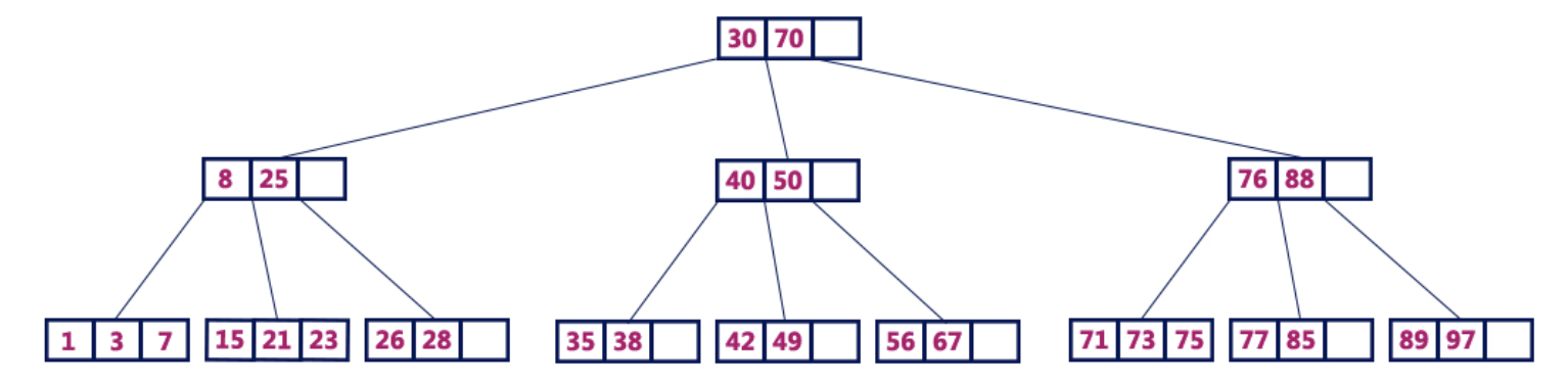
4-order B-tree
Operations on a B-tree The
following operations can be performed on a B-tree :
Searching the B-tree
Searching the B-tree is similar to searching the binary search tree. In the binary search tree, the search starts from the root and each time a two-way decision is made (go along the left subtree or right). In the B-tree, the search also starts from the root node, but at each step an n-sided decision is made, where n is the total number of descendants of the node in question. In the B-tree, the search complexity is O (log n) . The search is as follows:
Step 1: Read the item to search.
Step 2: Compare the searched item with the first key value in the root node of the tree.
Step 3: If they match, print: “The desired node was found!” And complete the search.
Step 4:If they do not match, check for more or less element value than the current key value.
Step 5: If the item you are looking for is smaller, continue searching the left subtree.
Step 6: If the desired item is larger, compare the item with the next key value in the node and repeat Steps 3, 4, 5 and 6 until a match is found or until the searched item is compared with the last key value in the leaf node.
Step 7: If the last key value in the list node did not match the search, print “Item not found!” And complete the search.
Insert operation in a B-tree
In a B-tree, a new element can only be added to a leaf node. This means that a new key-value pair is always added only to the leaf node. The insert is as follows:
Step 1: Check if the tree is empty.
Step 2: If the tree is empty, create a new node with a new key value and take it as the root node.
Step 3: If the tree is not empty, find a suitable leaf node to which a new value will be added using the logic of the binary search tree.
Step 4: If there is an empty cell in the current leaf node, add a new key-value to the current leaf node, following the increasing order of the key values inside the node.
Step 5: If the current node is full and does not have free cells, split the leaf node by sending the average value to the parent node. Repeat the step until the value to be sent is committed to the node.
Step 6:If the separation occurs with the root of the tree, then the average becomes the new root of the tree and the height of the tree increases by one.
Example:
Let's create a B-tree of order 3, adding numbers from 1 to 10.
Insert (1):
Since “1” is the first element of the tree, it is inserted into a new node and this node becomes the root of the tree.

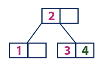
Insert (2):
The “2” element is added to an existing leaf node. Now we have only one node, therefore it is both the root and the leaf at the same time. This sheet has an empty cell. Then “2” gets into this empty cell.

Insert (3):
Element 3 is added to an existing leaf node. Now we have only one node, which is both the root and the leaf. This sheet does not have an empty cell. Therefore, we separate this node by sending the average value (2) to the parent node. However, the current node does not have a parent node. Therefore, the average value becomes the root node of the tree.

Insert (4):
Element “4” is larger than the root node with a value of “2”, while the root node is not a leaf. Therefore, we move along the right subtree of "2". We come to the leaf node with the value “3”, which has an empty cell. Thus, we can insert the “4” element into this empty cell.
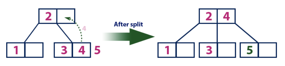
Insert (5):
Element “5” is larger than the root node with the value “2”, while the root node is not a leaf. Therefore, we move along the right subtree of "2". We come to the leaf node and find that it is already full and does not have empty cells. Then we divide this node by sending the average value (4) to the parent node (2). The parent node has an empty cell for it, so the value "4" is added to the node in which there is already a value of "2", and a new element "5" is added as a new sheet.
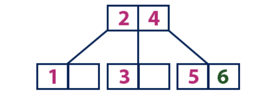
Insert (6):
The element “6” is larger than the elements of the root “2” and “4”, which is not a sheet. We move along the right subtree of the element "4". We reach a sheet with a value of "5", which has an empty cell, so the element "6" is placed just in it.
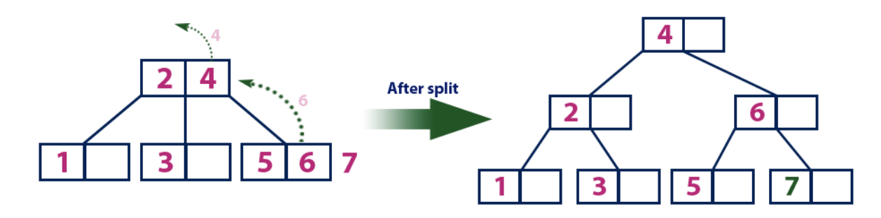
Insert (7):
The element "7" is larger than the elements of the root "2" and "4", which is not a leaf. We move along the right subtree of the element "4". We reach the leaf node and see that it is full. We divide this node by sending the average value of “6” up to the parent node with the elements “2” and “4”. However, the parent node is also full, so we divide the node with the elements “2” and “4”, sending the value “4” to the parent node. Only this node is not there yet. In this case, the node with the element “4” becomes the new root of the tree.
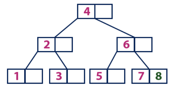
Insert (8):
Element 8 is larger than the root node with a value of 4, and the root node is not a leaf. We move along the right subtree from the element “4” and come to the node with the value “6”. “8” is greater than “6” and the node with the element “6” is not a sheet, so we move along the right subtree of “6”. We reach the leaf node with "7", which has an empty cell, so we put "8" in it.
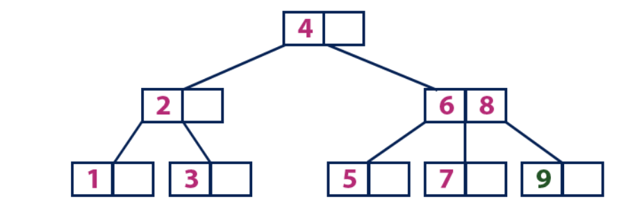
Insert (9):
Element 9 is larger than the root node with a value of 4, and the root node is not a leaf. We move along the right subtree from the element “4” and come to the node with the value “6”. “9” is greater than “6” and the node with the element “6” is not a sheet, so we move along the right subtree of “6”. We reach the leaf node with the values "7" and "8". He is full. We divide this node by sending the average value (8) to the parent node. The parent node “6” has an empty cell, so we put “8” in it. In this case, a new element "9" is added to the node list.
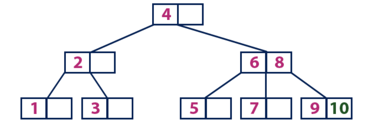
Insert (10):
The element "10" is larger than the root node with the value "4", while the root node is not a leaf. We move along the right subtree from the element “4” and come to the node with the values “6” and “8”. “10” is greater than “6” and “8” and the node with these elements is not a sheet, so we move along the right subtree of “8”. We reach the leaf node with a value of "9". He has an empty cell, so we put "10" there.
We suggest that you independently understand in practice how B-trees are arranged using this visualization .
We are waiting for everyone at a free open lesson , which will be held on July 12. See you!
In search trees, such as binary search tree, AVL tree, red-black tree, etc. each node contains only one value (key) and a maximum of two descendants. However, there is a special type of search tree called the B-tree (pronounced Bi-tree). In it, the node contains more than one value (key) and more than two descendants. The B-tree was developed in 1972 by Bayer and McCrate and was called the Height Balanced m-way Search Tree . Its modern name B-tree received later.
A B-tree can be defined as follows:
A B-tree is a balanced search tree in which each node contains many keys and has more than two children.
Here, the number of keys in the node and the number of its descendants depends on the order of the B-tree. Each B-tree has an order.
A B-tree of order m has the following properties:
Property 1: The depth of all leaves is the same.
Property 2: All nodes except the root must have at least (m / 2) - 1 keys and a maximum of m-1 keys.
Property 3: All nodes without leaves, except the root (i.e., all internal nodes), must have a minimum of m / 2 descendants.
Property 4:If the root is a leafless node, it must have at least 2 descendants.
Property 5: A node without leaves with n-1 keys must have n children.
Property 6: All keys in the node should be arranged in ascending order of their values.
For example, a 4-order B-tree contains a maximum of 3 key values and a maximum of 4 children for each node.
4-order B-tree
Operations on a B-tree The
following operations can be performed on a B-tree :
- Search
- Insert
- Delete
Searching the B-tree
Searching the B-tree is similar to searching the binary search tree. In the binary search tree, the search starts from the root and each time a two-way decision is made (go along the left subtree or right). In the B-tree, the search also starts from the root node, but at each step an n-sided decision is made, where n is the total number of descendants of the node in question. In the B-tree, the search complexity is O (log n) . The search is as follows:
Step 1: Read the item to search.
Step 2: Compare the searched item with the first key value in the root node of the tree.
Step 3: If they match, print: “The desired node was found!” And complete the search.
Step 4:If they do not match, check for more or less element value than the current key value.
Step 5: If the item you are looking for is smaller, continue searching the left subtree.
Step 6: If the desired item is larger, compare the item with the next key value in the node and repeat Steps 3, 4, 5 and 6 until a match is found or until the searched item is compared with the last key value in the leaf node.
Step 7: If the last key value in the list node did not match the search, print “Item not found!” And complete the search.
Insert operation in a B-tree
In a B-tree, a new element can only be added to a leaf node. This means that a new key-value pair is always added only to the leaf node. The insert is as follows:
Step 1: Check if the tree is empty.
Step 2: If the tree is empty, create a new node with a new key value and take it as the root node.
Step 3: If the tree is not empty, find a suitable leaf node to which a new value will be added using the logic of the binary search tree.
Step 4: If there is an empty cell in the current leaf node, add a new key-value to the current leaf node, following the increasing order of the key values inside the node.
Step 5: If the current node is full and does not have free cells, split the leaf node by sending the average value to the parent node. Repeat the step until the value to be sent is committed to the node.
Step 6:If the separation occurs with the root of the tree, then the average becomes the new root of the tree and the height of the tree increases by one.
Example:
Let's create a B-tree of order 3, adding numbers from 1 to 10.
Insert (1):
Since “1” is the first element of the tree, it is inserted into a new node and this node becomes the root of the tree.
Insert (2):
The “2” element is added to an existing leaf node. Now we have only one node, therefore it is both the root and the leaf at the same time. This sheet has an empty cell. Then “2” gets into this empty cell.
Insert (3):
Element 3 is added to an existing leaf node. Now we have only one node, which is both the root and the leaf. This sheet does not have an empty cell. Therefore, we separate this node by sending the average value (2) to the parent node. However, the current node does not have a parent node. Therefore, the average value becomes the root node of the tree.
Insert (4):
Element “4” is larger than the root node with a value of “2”, while the root node is not a leaf. Therefore, we move along the right subtree of "2". We come to the leaf node with the value “3”, which has an empty cell. Thus, we can insert the “4” element into this empty cell.
Insert (5):
Element “5” is larger than the root node with the value “2”, while the root node is not a leaf. Therefore, we move along the right subtree of "2". We come to the leaf node and find that it is already full and does not have empty cells. Then we divide this node by sending the average value (4) to the parent node (2). The parent node has an empty cell for it, so the value "4" is added to the node in which there is already a value of "2", and a new element "5" is added as a new sheet.
Insert (6):
The element “6” is larger than the elements of the root “2” and “4”, which is not a sheet. We move along the right subtree of the element "4". We reach a sheet with a value of "5", which has an empty cell, so the element "6" is placed just in it.
Insert (7):
The element "7" is larger than the elements of the root "2" and "4", which is not a leaf. We move along the right subtree of the element "4". We reach the leaf node and see that it is full. We divide this node by sending the average value of “6” up to the parent node with the elements “2” and “4”. However, the parent node is also full, so we divide the node with the elements “2” and “4”, sending the value “4” to the parent node. Only this node is not there yet. In this case, the node with the element “4” becomes the new root of the tree.
Insert (8):
Element 8 is larger than the root node with a value of 4, and the root node is not a leaf. We move along the right subtree from the element “4” and come to the node with the value “6”. “8” is greater than “6” and the node with the element “6” is not a sheet, so we move along the right subtree of “6”. We reach the leaf node with "7", which has an empty cell, so we put "8" in it.
Insert (9):
Element 9 is larger than the root node with a value of 4, and the root node is not a leaf. We move along the right subtree from the element “4” and come to the node with the value “6”. “9” is greater than “6” and the node with the element “6” is not a sheet, so we move along the right subtree of “6”. We reach the leaf node with the values "7" and "8". He is full. We divide this node by sending the average value (8) to the parent node. The parent node “6” has an empty cell, so we put “8” in it. In this case, a new element "9" is added to the node list.
Insert (10):
The element "10" is larger than the root node with the value "4", while the root node is not a leaf. We move along the right subtree from the element “4” and come to the node with the values “6” and “8”. “10” is greater than “6” and “8” and the node with these elements is not a sheet, so we move along the right subtree of “8”. We reach the leaf node with a value of "9". He has an empty cell, so we put "10" there.
We suggest that you independently understand in practice how B-trees are arranged using this visualization .
We are waiting for everyone at a free open lesson , which will be held on July 12. See you!