April 27, 2018 at 14:18
Mustache, paws and tail: how a neural network recognizes fur seals and other objects
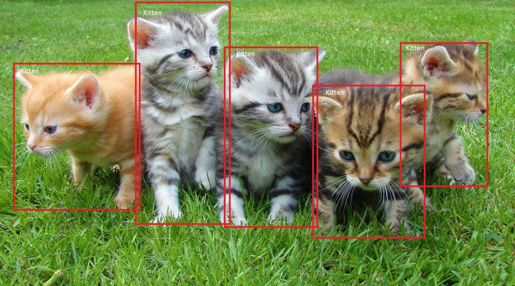
Image recognition is a classic example of the use of neural networks. Let us recall how the process of learning a network occurs, what difficulties arise and why use biology in development. Details under the cut.
Dmitry Soshnikov, Microsoft technical evangelist, member of the Russian Association of Artificial Intelligence, a teacher of functional and logical programming of AI at MAI, MIPT and HSE, as well as our courses, will help us in the story .
Imagine that we have many pictures that need to be sorted in two stacks using a neural network. How can this be done? Of course, it all depends on the objects themselves, but we can always highlight some features.
We need to know as much information as possible about the input data and take it into account at the manual entry, even before learning the network. For example, if we have the task of detecting multi-colored cats in the picture, not the color, but the shape of the object will be important. When we get rid of color, moving to a black and white image, the network will learn much faster and more successfully: it will have to recognize several times less information.
To recognize arbitrary objects, such as cats and frogs, color is obviously important: the frog is green, and cats are not. If we leave color channels, for each palette, the network learns to re-recognize image objects, because this color channel is fed to other neurons.
And if we want to destroy the famous meme about cats and bread, by teaching the neural network to detect an animal in any picture? It would seem that the color and shape are approximately the same. What to do then?
Filter banks and biological vision
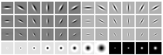
Using different filters, you can select different fragments of the image, which are then detected and examined as separate properties. For example, apply to traditional machine learning or neural networks. If the neural network has additional information about the structure of the objects with which it works, then the quality of work increases.
In the field of machine vision, filter banks have been developed - filter sets to highlight the main features of objects.
A similar “architecture” is also used in biology. Scientists believe that human vision does not determine the whole image, but highlights the characteristic features, unique features by which the brain identifies the object. Accordingly, for the quick and correct recognition of an object, it is possible to determine the most unique features. For example, in cats it can be a mustache - fan-shaped horizontal lines in the image.
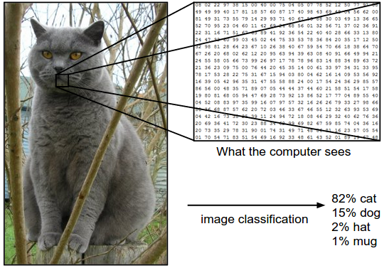
Weight Sharing
So that the network does not have to learn to separately recognize cats in different parts of the picture, we “divide” the weights responsible for recognition between different fragments of the input signals.
This requires a specialized network architecture:
- convolutional networks for working with images
- recurrence networks for working with text / sequences
Neural networks that are effectively used in image recognition, which use special convolution layers (Convolution Layers).
The basic idea is as follows:
- Use weight sharing to create a “filter window” that runs through the image.
- The filter applied to the image helps highlight fragments that are important for recognition.
- While in traditional machine vision, filters were designed by hand, neural networks allow us to design optimal filters through training
- Image filtering can naturally be combined with neural network computing.
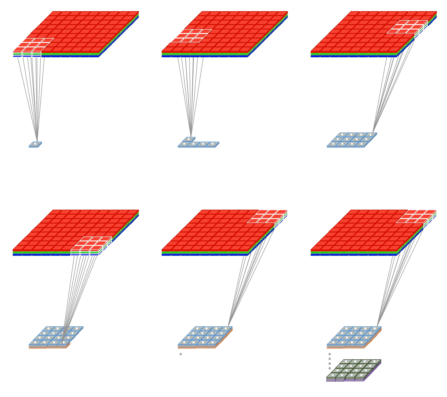
For image processing, convolution is used, as in signal processing.
We describe the convolution function with the following parameters:
- kernel - convolution kernel, weight matrix
- pad - how many pixels to add to the image at the edges
- stride - frequency of the filter. For example, for stride = 2, we will take every second pixel of the image vertically and horizontally, reducing the resolution by half
In [1]:
def convolve(image, kernel, pad = 0, stride = 1):
    rows, columns = image.shape
    output_rows = rows // stride
    output_columns = columns // stride
    result = np.zeros((output_rows, output_columns))
    if pad > 0:
        image = np.pad(image, pad, 'constant')
    kernel_size = kernel.size
    kernel_length = kernel.shape[0]
    half_kernel = kernel_length // 2
    kernel_flat = kernel.reshape(kernel_size, 1)
    offset = builtins.abs(half_kernel-pad)
    for r in range(offset, rows - offset, stride):
        for c in range(offset, columns - offset, stride):
            rr = r - half_kernel + pad
            cc = c - half_kernel + pad
            patch = image[rr:rr + kernel_length, cc:cc + kernel_length]
            result[r//stride,c//stride] = np.dot(patch.reshape(1, kernel_size), kernel_flat)
    return result
In [2]:
def show_convolution(kernel, stride = 1):
    """Displays the effect of convolving with the given kernel."""
    fig = pylab.figure(figsize = (9,9))
    gs = gridspec.GridSpec(3, 3, height_ratios=[3,1,3])
    start=1
    for i in range(3):
        image = images_train[start+i,0]
        conv = convolve(image, kernel, kernel.shape[0]//2, stride)
        ax = fig.add_subplot(gs[i])
        pylab.imshow(image, interpolation='nearest')
        ax.set_xticks([])
        ax.set_yticks([])
        ax = fig.add_subplot(gs[i + 3])
        pylab.imshow(kernel, cmap='gray', interpolation='nearest')
        ax.set_xticks([])
        ax.set_yticks([])
        ax = fig.add_subplot(gs[i + 6])
        pylab.imshow(conv, interpolation='nearest')
        ax.set_xticks([])
        ax.set_yticks([])
    pylab.show()
In [3]:
blur_kernel = np.array([[1, 4, 7, 4, 1],
                        [4, 16, 26, 16, 4],
                        [7, 26, 41, 26, 7],
                        [4, 16, 26, 16, 4],
                        [1, 4, 7, 4, 1]], dtype='float32')
blur_kernel /= 273
Filters
Blur
The blur filter allows you to smooth out irregularities and emphasize the overall shape of objects.

In [4]:
show_convolution(blur_kernel)
Vertical edges
You can come up with a filter that emits vertical brightness transitions in the image. Here, blue indicates the transition from black to white, yellow - vice versa.
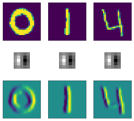
In [5]:
vertical_edge_kernel = np.array([[1, 4, 0, -4, 1],
                                   [4, 16, 0, -16, -4],
                                   [7, 26, 0, -26, -7],
                                   [4, 16, 0, -16, -4],
                                   [1, 4, 0, -4, -1]], dtype='float32')
vertical_edge_kernel /= 166
In [6]:
show_convolution(vertical_edge_kernel)
Horizontal edges
A similar filter can be built to highlight horizontal strokes in the image.
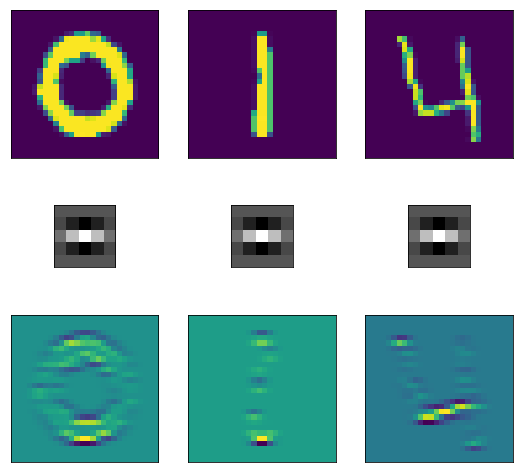
In [7]:
horizontal_bar_kernel = np.array([[0, 0, 0, 0, 0],
                                 [-2, -8, -13, -8, -2],
                                 [4, 16, 26, 16, 4],
                                 [-2, -8, -13, -8, -2],
                                 [0, 0, 0, 0, 0]], dtype='float32')
horizontal_bar_kernel /= 132
In [8]:
show_convolution(horizontal_bar_kernel)
Loop filter
You can also build a 9x9 filter that will highlight the contours of the image.

In [9]:
blob_kernel = np.array([[0, 1, 1, 2, 2, 2, 1, 1, 0],
                       [1, 2, 4, 5, 5, 5, 4, 2, 1],
                       [1, 4, 5, 3, 0, 3, 5, 4, 1],
                       [2, 5, 3, -12, -24, -12, 3, 5, 2],
                       [2, 5, 0, -24, -40, -24, 0, 5, 2],
                       [2, 5, 3, -12, -24, -12, 3, 5, 2],
                       [1, 4, 5, 3, 0, 3, 5, 4, 1],
                       [1, 2, 4, 5, 5, 5, 4, 2, 1],
                       [0, 1, 1, 2, 2, 2, 1, 1, 0]], dtype='float32')
blob_kernel /= np.sum(np.abs(blob_kernel))
In [10]:
show_convolution(blob_kernel)
Thus, a classic example with the recognition of numbers works: each digit has its own characteristic geometric features (two circles - eight, slash half the image - one, etc.), by which the neural network can determine what kind of object. We create filters that characterize each digit, run each of the filters in the image and minimize the error.
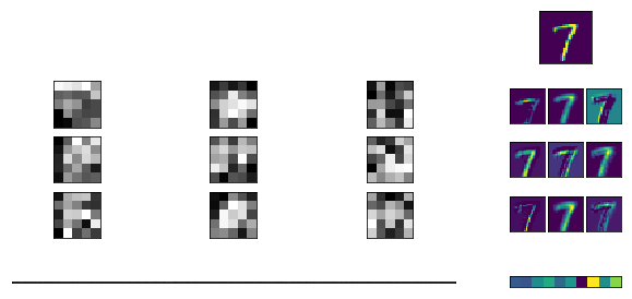
If you apply a similar approach to the search for cats in the picture, it quickly becomes clear that the four-legged has lots of signs for training the neural network, and they are all different: tails, ears, mustaches, noses, wool and coloring. And each cat can have nothing to do with the other. A neural network with a small amount of data on the structure of the object will not be able to understand that one cat is lying, and the second is on its hind legs.
The main idea of the convolution network
- Create a convolutional layer in the neural network, which ensures the application of the filter to the image.
- We train the filter weights using the backpropagation algorithm
For example, we have an image i , 2 convolutional filters w with outputs o . Elements of the output image will be calculated as follows:

Weight training
The algorithm is as follows:
- A filter with the same weights applies to all pixels in the image.
- At the same time, the filter “runs through” the entire image.
- We want to train these weights (common to all pixels) using the backpropagation algorithm.
- To do this, reduce the application of the filter to a single matrix multiplication.
- Unlike a fully connected layer, there will be less training weights, and more examples.
- Trick - im2col
im2col
Let's start with the image x, where each pixel corresponds to a letter:

Then we will extract all fragments of the 3x3 image and place them in the columns of the large matrix X:

Now we can save the filter weights in a regular matrix, where each row corresponds to one convolution filter:

Then the convolution over the entire image turns into the usual matrix multiplication:

Image Analysis Issues
In the learning process, many pitfalls can arise: incorrect sampling on the second layer will ruin the entire learning process, it may not be large enough, because of which the network does not learn to identify all kinds of provisions for the features of the object.
There is a reverse situation: when the number of layers increases, the gradient attenuates, too many parameters appear, and the function may become stuck at a local minimum.
In the end, nobody canceled the curve code either.
In order to teach working with neural networks, to cope with its training and to determine where in practice it is possible to use machine learning, Dmitry Soshnikov and I developed a special Neuro Workshop course. Of course, it talks about how to solve the above problems.
Neuro Workshop will be held 2 times:
Choose a convenient day, come and ask Dmitry your questions.