Dynamic System Modeling: An Introduction to GNU Octave

Once upon a time there were smart, but very greedy people who wrote the wonderful Matlab program. They were smart because the program came out good and greedy because they loved money very much. They loved it so much that they took it for their Matlab, not only from serious uncles who earned money, but also from poor students who also couldn’t buy a dry crust of bread for. And the fairy tale would end soon and sadly, if the world weren’t without kind and smart people who wrote programs similar to matlab, although they worked at the very least, but for all comers it’s free. And open source. So the poor students themselves began to add those programs, and they began to work better and better every year. And then they all began to live, live, and make good ...

Introduction

Most scientists do not puzzle over how the numerical methods are arranged inside. They simply use them, using specialized packages of numerical calculations in their work. This does not mean at all that you do not need to understand how these methods work. A person writes a program, but it is a mistake for him. And errors are discernible even in the most expensive and sophisticated systems of numerical mathematics all the time. In addition, there are tasks where the use of standard systems is impossible.

At the same time, the ability to use universal mathematical software is a must have for a modern scientist, because when inventing a bicycle you can never get to solving your main problem. Today we will consider the promised Octave, trying to solve the next children's problem with its help, making non-childish conclusions.

1. What is Octave and where to get it

GNU Octave is a free math math package based on the concepts of its proprietary fellow Matlab. It is available for all currently popular desktop platforms, and you can get it by going to the download section on the official website.



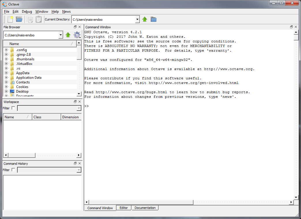
Most of the screen is occupied by the so-called command window, with a command prompt of the form ">>". We’ll enter something there and press Enter

>> 2 + 2
ans = 4

gorgeous, the variable ans contains the result of the last operation, unless you explicitly entered the variable under the result, for example

>> x = 3 + 2
x =  5

variables are entered on the fly, as is customary in interpreted languages. Yes, actually the m-language octave is the language of the interpreter, very reminiscent of a similar language matlaba. Once wound up, the variable retains its value and type until the next assignment, or until the shell is completely cleared

>> x + ans
ans =  9

On the left side of the window there is an area in which (top to bottom) are located: the file manager, a list of global variables with their values, as well as the history of the entered commands.



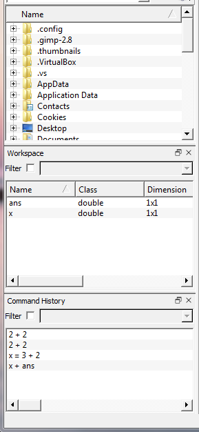
It is worth noting that for the variables the dimension (Dimention) 1x1 is indicated. The main data type in Octave, as in Matlab, is the matrix. So our numbers are actually matrices of 1 per 1 element size.

You can clear all global variables by choosing Edit -> Clear Workspace from the menu, and clear the command window by right-clicking on it, choosing Clear Window. We clean the variables and entering x we ​​get

>> x
error: 'x' undefined near line 1 column 1
>> x = 3
x =  3
>> x
x =  3

it can be seen that the variable x became unavailable until we explicitly assigned it a value again.

Frankly, I have never worked with Ocatve and I understand it with the reader. Therefore, suppose that we already know enough to solve some kind of problem. For example, the one that was decided last time . But first…

2. The normal form of Cauchy

Remember, I said that the majority, with the exception of a narrow class, of numerical methods are “sharpened” for first-order equations? And what before applying these methods to the solution of the equation, it is necessary to lower its order? The trouble is that not all equations allow lowering the order. However, any n-th order equation can be turned into n 1st-order equations. This is called the conversion of the equation to the normal Cauchy form . Take the past equation

$$

We recall that

$$

then

$$

and instead of one second-order equation, we get two first-order equations that need to be solved together, simultaneously

$$

This is not just one equation, but a system of differential equations containing two unknown dependencies $$ and $$.

How to solve the system of equations numerically? Yes, just like one equation. Let's collect all our variables in a column vector (either an array or a column matrix, for whom it is not convenient to express it)

$$

and the right parts are also collected in a column vector

$$

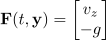
Then the recurrence formula of the Euler method will be valid for each element of these columns

$$

where n is the number of equations, in our case there are two of them.

Why am I doing all this? And the fact that Octave requires to represent differential equations in the normal Cauchy form.

From the point of view of mechanics, the column vector y is called the state vector of the system or the vector of phase coordinates . Then our system of equations turns into one vector equation

$$

Now take, and in the Octave command window, type

>> function dydt = F(y, t)

Thus, we define a function that receives the current value of the phase coordinates y and the current time t at the input , and returns the value of the derivatives of the phase coordinates at the output. We see that the command prompt ">>" is gone, the system waits for us to finish entering the function body with the endfunction keyword. Continue to dial the function

>> function dydt = F(y, t)
g = 10
dydt(1) = y(2)
dydt(2) = -g
endfunction

So, in the body of the function, we determined g = 10 - the accepted value of the acceleration of gravity. We see that it did not appear in the list of variables on the left - this variable is local, and exists only within the function. The variable y is the column matrix, the first element of y (1) of which is the coordinate z, and the second y (2) is the projection of the velocity vector v _z . Accordingly, dydt is the value that our function returns, it is also a column matrix, the first element of which is the derivative of z in time, and the second is the derivative of v _z in time. That is, we wrote down our system of differential equations in terms of Octave.

Now we decide on the time range for which we need to get the result. Let it be ten points from 0 to 1 second, with a step of 0.1 - compare the result with a manual example

>> t0 = 0
t0 = 0
>> tend = 1
tend =  1
>> deltaT = 0.1
deltaT =  0.10000
>> t = [t0:deltaT:tend]
t =
   0.00000   0.10000   0.20000   0.30000   0.40000   0.50000   0.60000   0.70000   0.80000   0.90000   1.00000

Everything is obvious here: t0 is the initial moment of time, tend is the final moment of time. But deltaT = 0.1 second is not an integration step ! This is the interval at which Ocatve will display for us a numerical solution to the equation. The last command forms an array of time points for which we want to get a solution.

As you know from the last article , to solve the equation numerically it is necessary to know the initial values ​​of velocity and coordinates. You must set them for Octave

>> y0 = [100; 0]
y0 =
   100
     0

thereby, we determined a column matrix containing the initial coordinate and the initial value of the vertical projection of velocity. Now we solve the equation

>> y = lsode("F", y0, t)

The lsode function solves the equation numerically for us. The first parameter is the name of the function that calculates the derivatives of the phase coordinates. This is function F, we defined it. The second parameter is the initial conditions , that is, the values ​​of the phase coordinates at time t = t0. The last parameter is an array of time points for which we want to calculate the values ​​of the phase coordinates. Press Enter ...

In response, a mountain of tripe falls out, ending with a sentence

g =  10
dydt = -0.99690
dydt =
   -0.99690  -10.00000
g =  10
dydt = -0.99690
dydt =
   -0.99690  -10.00000
g =  10
dydt = -0.99690
dydt =
   -0.99690  -10.00000
g =  10
dydt = -1.9936
-- less -- (f)orward, (b)ack, (q)uit

we are offered to flip through entrails further (f), go back (b), or exit (q). Those who know * nix-like systems know that this is console output under the control of the less unix utility. We pretend we don’t know, get out of here by pressing q on the keyboard.

Now type in the command line "y" and press Enter

>> y
y =
   100.00000     0.00000
    99.95000    -1.00000
    99.80000    -2.00000
    99.55000    -3.00000
    99.20000    -4.00000
    98.75000    -5.00000
    98.20000    -6.00000
    97.55000    -7.00000
    96.80000    -8.00000
    95.95000    -9.00000
    95.00000   -10.00000

Doesn’t resemble anything? Well, of course, this is the very solution that we got for the task from the previous article. Only now it is surprisingly accurate - the values ​​coincide with the analytical solution! I will tell you a secret - this is the exact solution to our problem. This is due to the fact that the lsode function does not use the Euler method to solve the problem, but something more advanced. The movement of the stone occurs with constant acceleration, and the numerical approximation formula that is used in this method obviously just coincides with the analytical solution to the problem. Although, if you climb into the wilds of a machine representing floating point numbers, then ... Well, oh well, now this is not about that.

3. Build a schedule

Type the command now

>> plot(t, y)

A window will pop up with a graphical representation of the solution. The



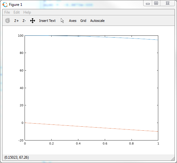
blue curve above is the coordinate of the stone. Orange below is a vertical projection of speed. The entered command is inconvenient in that it builds a graph for all functions at once. And if we want to build, the dependence of speed on height? Then we will do so

>> plot(y(:,1), y(:,2))

A graph will be constructed where the y (1) variable will go along the abscissa and y (2) along the ordinate, which is the height and vertical projection of speed, respectively.



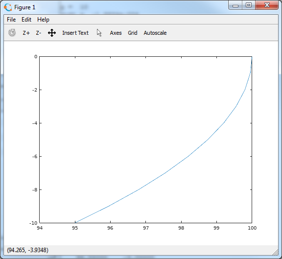
Such a graph in mechanics is called the phase portrait of the system , i.e. the trajectory of the system in the phase space coordinates. In this case, the phase coordinates are the height of the stone above the surface of the Earth and its speed. In mechanics it is often impossible to get an exact solution in the form of functions of time, but you can relate coordinates and speeds to each other based on energy considerations. Based on the obtained dependences, one can find the phase trajectory of the system and draw many conclusions about the nature of its movement without solving the problem to the end. We will also talk about this somehow.

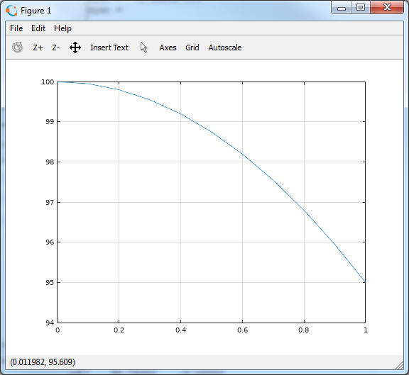
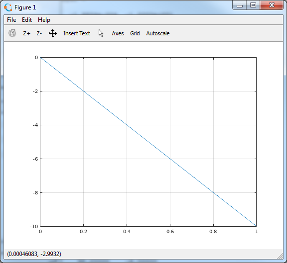
In the meantime, I propose to perform an independent task - build a graph of the dependence of height on time and speed on time in separate windows. And try not to look under the spoiler

Conclusion

This is the first acquaintance with Octave, as a medium for numerical simulation, we will consider complete. Now we have a powerful tool with which we will comprehend more sophisticated wisdom.

Thanks for watching, see you!