The magic of tensor algebra: Part 9 - Derivation of the angular velocity tensor through the parameters of the final rotation. Apply Maxima

maisvendoo July 16, 2015 at 23:06

The magic of tensor algebra: Part 9 - Derivation of the angular velocity tensor through the parameters of the final rotation. Apply Maxima

Content

Introduction

It has already leaked by the order of time, as I promised to obtain the angular velocity tensor of a solid, expressing it in terms of the parameters of the final rotation. If you look at the KDPV, it will become clear why I thought for so long - a stack of paper on the table is my train of thought.

The transformation of tensor expressions is still a pleasure ... The

brutal tensors did not want to simplify. Rather, they wanted it, but during the transformations, the disclosure of the brackets, due to inattention, minor errors occurred that did not allow us to look at the whole picture. As a result, the result was obtained. Not the last role in this was played by SKA Maxima, whom I turned to, largely thanks to an article by EugeneKalentev. The emphasis of this article was shifted toward computational work with tensors, the components of which are represented by specific data structures. I was interested in the issue of working with abstract tensors. It turned out that Maxima can work with them, although not the way it might be wanted, but still it seriously simplified my life.

So, we return to the mechanics of solids, and at the same time see how to work with tensors in Maxima.

1. A little about the final expression of the rotation tensor

In the last article, we, having studied the principles of convolution of the product of Levi-Civita tensors, got this expression for the rotation tensor

$B_k ^ {\, m} = u ^ {\, m} \, g_ {jk} \, u ^ {\, j} - \ cos \ varphi \, \ left (\ delta_ {j} ^ {\, m } \, \ delta_ {k} ^ {\, q} - \ delta_ {k} ^ {\, m} \, \ delta_ {j} ^ {\, q} \ right) \, u_ {q} \, u ^ j + \ sin \ varphi \, g ^ {mi} \, U_ {ik} \ right \ quad (1)$

It can be simplified yet, for this we’ll work with the expression in parentheses in the second term

$\ left (\ delta_ {j} ^ {\, m} \, \ delta_ {k} ^ {\, q} - \ delta_ {k} ^ {\, m} \, \ delta_ {j} ^ {\, q} \ right) \, u_ {q} \, u ^ j = \ delta_ {j} ^ {\, m} \, \ delta_ {k} ^ {\, q} \, u_ {q} \, u ^ j - \ delta_ {k} ^ {\, m} \, \ delta_ {j} ^ {\, q} \, u_ {q} \, u ^ j =$

$= u ^ m \, u_ {k} - \ delta_ {k} ^ {\, m} \, u ^ q \, u_ {q} = u ^ m \, u_ {k} - \ delta_ {k} ^ {\, m} \ quad (2)$

And all because the convolution of the tensor with the Kronecker delta leads to the replacement of the silent tensor index by the free index of the Kronecker delta, for example $\ delta_ {k} ^ {\, q} \, u_ {q} = u_ {k}$ . Acting in this way, and taking into account that the vector $\ vec {u}$ has a length equal to one, which means convolution $u ^ {q} \, u_ {q} = 1$ , we get (2). Then the expression of the rotation tensor looks even simpler

$B_k ^ {\, m} = \ left (1 - \ cos \ varphi \ right) u ^ {\, m} \, u _ {\, k} + \ cos \ varphi \, \ delta_ {k} ^ {\ , m} + \ sin \ varphi \, g ^ {mi} \, U_ {ik} \ right \ quad (3)$

just the expression that I tried for a long and tedious attempt to deduce in the seventh article . Which once again confirms the rule that you can’t study anything by half ...

Why did I do all this. First, to finally rehabilitate in the eyes of readers. Secondly, so that we have something to compare the results that we get a little lower with Maxima. And thirdly, to say that on expression (3) our sweet life ends and the hell of monstrous transformations begins.

2. We use Maxima to derive the angular velocity tensor

A module is responsible for working with abstract tensors in Maxima itensor, the documentation for which is presented in the original , translated into Russian , and another book based on documentation.

We launch Maxima, at least in the console, at least using one of its graphic frontends, and write

kill(all);
load(itensor);
imetric(g);
idim(3);

Here we clean the memory (function kill()), removing all definitions and loaded modules from it, load the package itensor(function load()), say that the metric tensor will be called g(function imetric()), and we also specify the space dimension (function idim()), because by default SKA believes that it works in 4-dimensional space-time with the Riemann metric. We are working in the three-dimensional space of classical mechanics, and our metric is any torsion-free non-degenerate.

We introduce the rotation tensor

B:ishow( u([],[l])*g([j,k],[])*u([],[j]) - 
cos(phi)*'levi_civita([],[l,q,i])*u([q],[])*'levi_civita([i,j,k],[])*u([],[j]) + 
sin(phi)*g([],[l,i])*'levi_civita([i,j,k])*u([],[j]))$

The itensortensors are declared by the identifier, after which the lists of covariant and contravariant indices are indicated in brackets with a comma. The function levi_civita()defines the Levi-Civita tensor, and the prime in front of it means that this tensor does not need to be calculated. Maxima is known for her way of calculating and simplifying expressions if possible, and if the stroke is not put, then the Levi-Civita tensor will turn into a “pumpkin”, and specifically, an attempt will be made to determine it through the generalized Kronecker delta, which is not included in our plans.

The symbol $is an alternative to a semicolon and prohibits the display of conversion results on the screen. To display information we will useishow(). The expression substituted into it is displayed on the screen in the usual index notation of the tensor record. On the screen, it looks like this.

Moreover, we introduce its non-simplified form, with a double vector product, without introducing an antisymmetric tensor $\ mathbf {U}$ , in order to obtain (3) at the first stage and check how the machine simplifies tensor expressions. In human terms, this expression looks like this

$g_ {j \, k} \, u ^ {l + j} - \ varepsilon_ {i \, j \, k} \, \ cos \ Phi \, \ varepsilon ^ {i \, l \, q} \, u_ {q} \, u ^ {j} + g ^ {i \, l} \, \ varepsilon_ {i \, j \, k} \, \ sin \ Phi \, u ^ {j}$

the truth is the sum of the indices in the first term suggests suspicion of some special magic that is unknown to us. But this conclusion is generated directly by Maxima, using the spell

load(tentex);
tentex(B);

which allows you to get output in the form of LaTeX code. Among the shortcomings - shamanism with indexes and a capital letter indicating the angle of rotation, but both of them are fixable in principle, but Maxima pleased me with the fact that TeX-output is not as redundant as Maple.

Move on. Next, we recall the expression that determines the angular velocity through the rotation tensor

$\ Omega _ {\, mk} = g _ {\, mp} \, B_ {l} ^ {'\, p} \, \ dot {B} _ {k} ^ {\, l} \ quad (4)$

Now imagine that we have to differentiate (3) with respect to time, then multiply the derivative by the inverse matrix (3) and the metric tensor. This can be done manually, but if I brought this process to the end, the stack of sheets on the table would be three times thicker.

First of all, we simplify the introduced rotation tensor

B:ishow(expand(lc2kdt(B)))$

The function is lc2kdt()designed specifically to simplify expressions containing the Levi-Civita tensor. She tries to collapse this tensor where possible, giving the output a combination of the sums and products of the Kronecker deltas. This is how the result looks . The function that opens the brackets is also applied

to the result . Without this, Maxima performs the convolution very reluctantly. Now let's try to calculate the resulting expression by doing a convolution. Function is one of the most reliable ways to perform convolution.lc2kdt()expand()

contract()

B01:ishow(contract(B))$

We get the output (where possible, I will give the LaTeX output generated by Maxima using the function tentex())

$\ delta_ {k} ^ {l} \, \ cos \ Phi \, u_ {q} \, u ^ {q} -u_ {k} \, \ cos \ Phi \, u ^ {l} + u_ {k } \, u ^ {l} + g ^ {i \, l} \, \ varepsilon_ {i \, j \, k} \, \ sin \ Phi \, u ^ {j}$

which is similar to expression (3). This convinced me of the correctness of the program and the correctness of my own actions. So you can move on.

The only thing Maxima does not take into account is that the vector around which the rotation is made has a length equal to one. Therefore, he does not collapse the expression $u ^ {q} \, u_ {q}$ into a scalar. How could I tell him about this I did not come up with and did not subtract this from the documentation, although I searched carefully. In the future, this will give serious difficulties, which we will talk about, but for now I got out with the help of a crutch, replacing the uncomfortable tensors with a unit

B01:ishow(subst(1, u([],[q]), B01))$
B01:ishow(subst(1, u([q],[]), B01))$

The expression of the rotation tensor in terms of the parameters of the final rotation has the pleasant property that obtaining the inverse matrix reduces to substituting the rotation angle with the opposite sign in (3). Indeed, turning in the other direction is the inverse transformation. This can be proved strictly mathematically, based on the properties of the rotation matrix. I have done this and consider it unnecessary leads in this article. Just get the inverse tensor

B10:ishow(subst(-phi, phi, B01))$

Since we are going to take the derivative, then Maxima should know which tensors and numerical parameters depend on time. We indicate that the direction of the axis of rotation and the angle of rotation depend on time

depends([u,phi], t);

So that our tensors correspond to formula (4), we rename the indices

B10:ishow(subst(p,l,B10))$
B10:ishow(subst(l,k,B10))$
B10:ishow(subst(i1,i,B10))$
B10:ishow(subst(j1,j,B10))$
B10:ishow(subst(s,q,B10))$

Thus, we changed the names of free indexes for correct multiplication in (4), and redefined the names of silent indexes. According to the rules, it is assumed that the names of the silent indexes in the multiplied tensors do not coincide.

Now we take the time derivative of the rotation tensor

dBdt:ishow(diff(B01,t))$

getting the output

We are convinced that the differentiation was performed correctly. Finally, we introduce formula (4), applying successively the disclosure of the brackets and simplification taking into account the Levi-Civita tensor

exp1:ishow(lc2kdt(expand(g([m,p],[])*B10*dBdt)))$

The result is scary to show, but if you please,

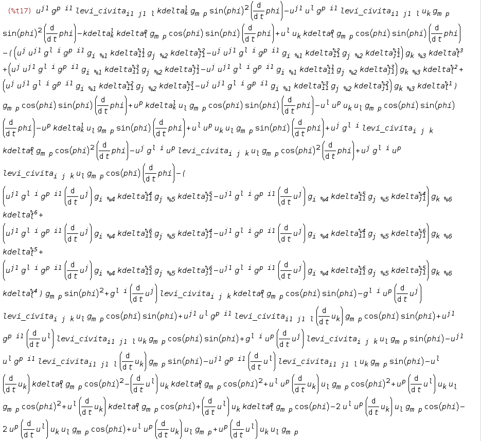
it’s difficult to understand anything in this mess. But it is clear that combinations of the Kronecker deltas (the function kdelta()sets the Kronecker delta of any desired rank) with a strange notation of dumb indices containing the number after got out %. The fact is that Maxima, when transforming, numbers dumb indices. Let's try to simplify all this

First, once again, let's run the expression through simplification taking into account the Levi-Civita tensor ( lc2kdt()). Then do the convolution ( contract()). After that, we will try to simplify our “crocodile” by applying a function to it canform()that performs the numbering of silent indexes and simplifies the tensor. This feature is recommended by developers for simplifications.

exp2:ishow(canform(contract(lc2kdt(exp1))))$

As a result, we observe a serious weight loss of the "crocodile"

But! In the first term, we see the vector product of the unit vector of the axis of rotation of itself, and it should be equal to zero. Maxima has not yet understood this, she needs to point out the possibility of such a simplification. We make it a construction

exp3:ishow(canform(contract(expand(applyb1(exp2,lc_l,lc_u)))))$

The function applyb1()sets the rules for simplifying the subexpressions included in the simplified expression. An expression and a list of rules are passed as arguments. We have two rules : lc_land lc_u- the rules for converting subexpressions with the Levi-Civita symbol with lower ( lc_l) and upper ( lc_u) indices. At the same time, we again open the brackets that may appear after the conversion of subexpressions, we perform convolution and simplification. As a result, we observe another reduction in crocodile mass.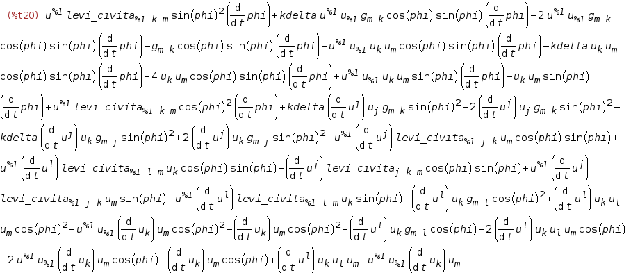

Perhaps this is not the limit. But I was surprised, probably by ignorance and lack of experience, the following

Let's pay attention to the variable kdelta. The experiments with Maxima made it possible to find out that this is a trace of the Kronecker delta of rank 2, equal to the dimension of space (trace of a single matrix). In our case, this is the number "3". It is the three that must stand still kdelta. But for some reason it’s not worth it, maybe the tensor package configuration variables are somehow incorrectly configured. If we take it kdeltaequal to three, then a bunch of similarly similar terms are formed, which in total give zero.
All view convolutions
$u ^ {i} \, u_ {i}$

This is the unit of rotation unit, but it does not change and is equal to unity. How to say this about Maxima has not yet been clarified for me.
It flows from the previous problem, for
$u ^ i \, u_i = 1$

which means

$\ dot u ^ {i} \, u_ {i} + u ^ {i} \, \ dot u_ {i} = 0 "$

whence, due to the commutativity of the scalar multiplication operation, we have

$\ dot u ^ {i} \, u_ {i} = 0, \ quad u ^ {i} \, \ dot u_ {i} = 0 "$

Recent expressions are often found in the above result.

I would be very grateful for the help of those who know about these problems, because studying the documentation has not yet shed light on the solution. The replacement function subst()does not work here.

In this regard, I again took up the pen and paper to "simplify" the angular velocity tensor. But Maxima greatly facilitated my task, for which she thanks.

3. Using a pen, paper, file and tambourine ...

We write out all nonzero terms, present similar ones, and take out the common factors out of brackets. Surprisingly, everything collapses beautifully and quickly into a formula

$\ Omega _ {\, km} = \ left (1 - \ cos \ varphi \ right) \ left (\ dot u _ {\, k} \, u _ {\, m} - u _ {\, k} \, \ dot u _ {\, m} \ right) + \ sin \ varphi \, \ left (1 - \ cos \ varphi \ right) \, u ^ {\, i} \ left (\ varepsilon _ {\, ijk} \, \ dot u ^ {\, j} \, u _ {\, m} - \ varepsilon _ {\, ilm} \, \ dot u ^ {\, l} \, u _ {\, k} \ right) +$

$+ \ sin \ varphi \ cos \ varphi \, \ dot u ^ {\, j} \ varepsilon _ {\, jkm} + \ dot \ varphi \, \ varepsilon _ {\, ikm} \, u ^ {i} \ quad (5)$

This expression painfully resembles a similar one obtained for an orthogonal basis and expressed in a matrix form

Pogorelov D. Yu. Introduction to modeling the dynamics of systems of bodies. Page 31.

Tensor (5) is antisymmetric, rearrange the indices, changing the signs of the corresponding expressions. The first term is the difference of the covariant tensor products, the second is the transposed first, and such a sum gives the output an antisymmetric tensor. The remaining terms contain the Levi-Civita tensor, which changes sign when the indices are rearranged

$\Omega_{\,mk} = \left(1 - \cos\varphi \right )\left(\dot u_{\,m} \, u_{\,k} - u_{\,m} \, \dot u_{\,k}\right ) + \sin\varphi \, \left(1 - \cos\varphi \right ) \, u^{\,i} \left( \varepsilon_{\,ilk} \, \dot u^{\,l} \, u_{\,m} - \varepsilon_{\,ijm} \, \dot u^{\,j} \, u_{\,k} \right ) +$

$- \sin\varphi \cos\varphi \, \dot u^{\,j} \varepsilon_{\,jmk} - \dot\varphi \, \varepsilon_{\,imk} \, u^{i}$

And again, we rearrange the indices in the last two terms

$+ \sin\varphi \cos\varphi \, \varepsilon_{\,mjk} \, \dot u^{\,j} + \dot\varphi \, \varepsilon_{\,mik} \, u^{i} \quad (6)$

so that their convolution gives skew-symmetric matrices, which are familiar for representing a vector product in matrix form.

Further simplification (6) is possible if the basis is Cartesian. Then the covariant and contravariant components coincide, the nonzero elements of the Levi-Chevita tensor modulo become equal to unity, and (6) can be simplified a little more. But we got this expression for an arbitrary basis.

Conclusion

So, thanks to the Maxima tensor tools, I finally figured out the task of expressing the angular velocity tensor through the parameters of the final rotation. At the same time, he showed the reader a living example of working with tensors in SKA.

Next time, we obtain from (6) the pseudovectors of angular velocity and angular acceleration and come close to the tensor description of the kinematics of a solid.

Thank you for attention!

To be continued…

Tags:

The magic of tensor algebra: Part 9 - Derivation of the angular velocity tensor through the parameters of the final rotation. Apply Maxima