July 9, 2015 at 15:45
Using potential fields in a real-time strategy scenario
- Transfer
Implementing unit behavior in RTS games can be a serious problem. The computer often controls a huge number of units, including those belonging to the player, which must move in a large dynamic world, simultaneously avoiding collisions with each other, looking for enemies, protecting their own bases and coordinating attacks to destroy the enemy. Real-time strategies work in real time, which makes it rather difficult to track action planning and navigation.
This lesson describes a game flow planning and unit navigation method that uses multi-agent potential fields. It is based on works under the numbers [1, 2, 3]. (See the end of the article for links to the materials used)

PP (Potential Field) has a number of similarities with influence maps. Influence cards are often used to determine whether a zone in the game world is under the control of a player or enemies (in the range of weapons or movement range), or is it a zone that is not currently controlled by anyone (no one’s land). The idea is to put positive values on the cells under the control of the player, and negative values under the control of the enemy. By smoothly decreasing the value to zero, we will create a map that reflects the influence of our and enemy units in the zone. The figure below shows an example of a map of influence with one of its own and one enemy unit.

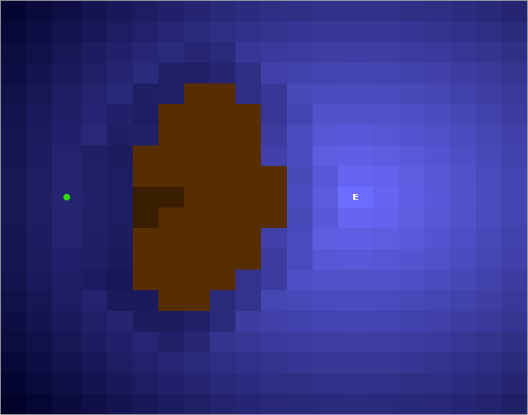
Potential fields work in a similar way - a charge is put on an interesting position in the game world and generates a field that gradually goes to zero. The charge can be attractive (positive) or repulsive (negative). Note that in some literature on potential fields, negative charges are attractive and vice versa. In this lesson, positive charges are always hiding. The figure below shows a simple game world with some impassable territory (brown), an enemy unit (green) and the destination of the unit (E). The attracting charge is located at the destination.

The charge generates a field that spreads through the game world:
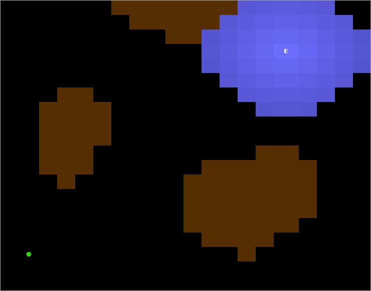
And fades to zero:

In the illustration above, the attractive field has spread around the destination point “E”. The point is to let the green unit move to the positions with the most attracted values and finally find the way to the destination. To make this work, we also need to deal with obstacles in the game world, in this case with mountains (cinnamon zones). If we force the mountains to generate small repulsive fields and add them to the attracting fields (from the figure above), we get a resulting field that can be used for navigation. Since units always move to a neighboring position with the most attractive value, we will go around the mountains if there is another way.
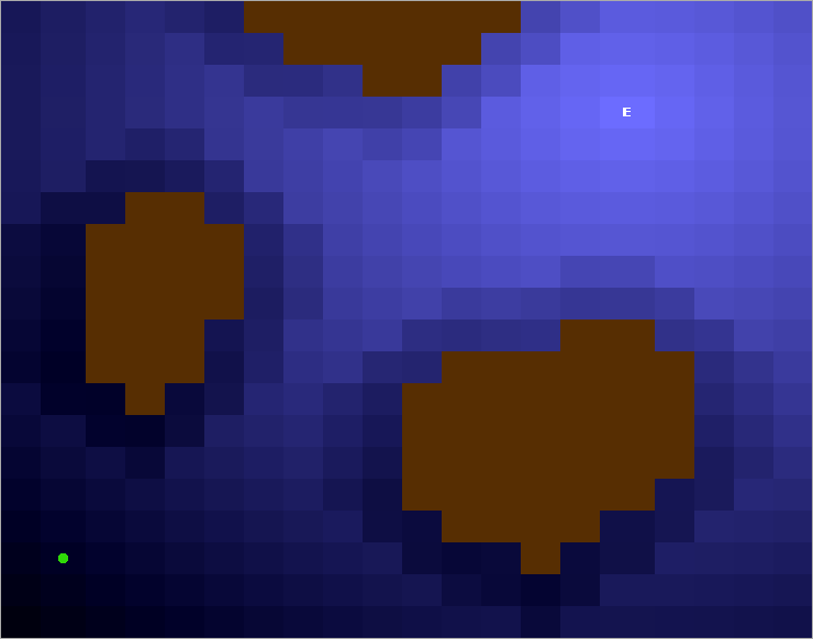
The same idea is used for other obstacles. In the picture below, two more of their units (white) were added. They generate small repulsive fields, which again add up to the resulting field.

Thus, our green unit will bypass these units to avoid a collision. Now we have got the final path for our unit. A unit can move from its current position to its destination and bypass all obstacles without using any algorithm for finding the path.
One of the main advantages of using potential fields is the ability to process dynamic game worlds. Since units (agents) move only one step at a time, instead of generating a full path from A to B, there is no risk that the path will become unavailable due to changes in the game world. Finding a path in a dynamic world can often be difficult to implement and require a lot of resources to calculate. When an approach based on potential fields is used, the solution to the problem comes automatically. Of course, you need to be careful when implementing the PP system, so as not to forget to make updating potential fields as effective as possible. (More about this later).
Another important advantage is the ability to create complex behavior by simply playing with the shape settings of the generated fields. Instead of linear attenuation to zero, we can use nonlinear fields. If, for example, we have shooting units like tanks in our army, we don’t want the tanks to move too close to the enemy units, but surround them at the right distance (for example, at the distance of their firing range). This behavior can be achieved by placing a zero charge at the location of the enemy unit, generating an increasing field with the most attracted point at the firing range, and then fading to zero. The picture below shows an example with two tanks (green) moving in an attack on an enemy unit (red), generating a non-linear PP.

An example of the equation of how such a field can be generated:

Here W1 is the value for changing the relative strength of the field. D is the maximum firing range and R is the maximum detection range (from where our agent sees the enemy agent).
Another behavior that is easy to implement is “kick-run”. First, the unit approaches the maximum attack distance.
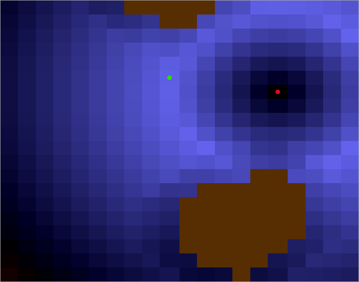
After the attack, our unit must reload its weapon and retreats from the enemy unit until it is ready to shoot again.

During the retreat phase, all enemy units generate a strong repulsive field with a radius of the maximum range of the unit. This is an example of how specific potential fields can be active or inactive depending on the internal state of the agent controlling this unit. An inactive field is simply ignored when the resulting potential field is summed.
The image below is a screenshot of our software- based bot for ORTS.engine. The left side of the image is a 2D view of the current state of the game. It shows our tanks (green circles) going to attack enemy bases (red squares) and units (red circles). Brown and black zones - impassable territory (mountains). The potential field of this game state is shown on the right side of the image. As in other pictures from this lesson, the blue zones are the most attractive. The light lines are the attacks of our tanks. The PP view clearly shows how our units surround the enemy at the maximum range of the shot, while avoiding collisions with each other and the terrain. The behavior of the environment of the enemy works fine and was perhaps one of the key in our success of 2008 at the ORTS tournament.

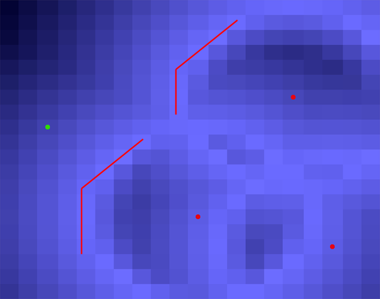
While we were developing our bot for ORTS, we discovered one thing - a completely different behavior when summing the potentials of enemy units generated at each point was compared with simply the highest potential of the enemy unit at that point. In the figure below, the potentials generated by three enemy units are summed up and added to the resulting field. Thus, the greatest potential is directly in the center of the enemy unit cluster (circled in red) and our units were very keen to attack the enemies at their strongest points.

The solution was not to summarize the potentials, but instead to take the greatest potential at a point from all units. In the latter case, the highest potential around the enemies at an acceptable distance (shown by red lines).
With a good plan and implementation of the PP system, the cost of resources for calculation will not exceed traditional solutions based on the A * algorithm. Our ORTS bot used the least amount of CPU resources compared to two other bots working on path search algorithms since the 2007 tournament. However, we note that it is difficult to accurately calculate the CPU usage due to the fact that the winning bot uses more resources at the end of the game, as it has more units under control. Multithreading also complicates the task of calculating the required CPU resources. The comparison was carried out by comparing the total amount of CPU resources used by each client process in the Linux environment for 100 games. At least we can conclude that the bot was good within the allotted time of 0.125 seconds used in ORTS.
To improve performance, we divided software into three categories:
We experimented with two main architectures for generating PP ...
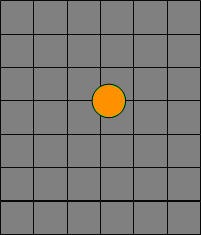
The field generated by each type of object was previously calculated and stored in static arrays in the header file. During the execution of the program, these fields were simply added to the general software at the desired position. To make this possible, the game world was divided into tiles, in our case, each tile consisted of 8x8 points of the game world. This approach showed insufficient detail and the bot performed poorly (2007 ORTS tournament). Since the game world was divided into significantly larger tiles, we ran into problems deciding which tile (which tiles) an object occupies. Assume an object (orange circle) and a base (orange square). What tiles (gray squares) does our green unit occupy and what tiles should the base occupy?
This approach may be suitable for games like Wargus, which use a less detailed tile navigation system.

The potentials generated at the point are calculated in real time by calculating the distance between the point and all nearby objects, passing each distance as a variable to a function and then calculating the potential. This approach, in fact, uses less CPU resources in our bot than pre-generated fields.
Thanks to:
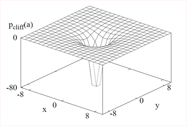
This approach was used in the second version of our bot (2008 ORTS tournament). An example of the PP formula (with 2D and 3D graphs) used to calculate the potential generated by a cliff at a point with a distance “a” from the cliff.


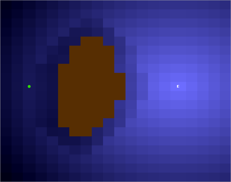
One of the most common problems with PP is the problem of local optimum. The picture below shows an example when this problem appears. Destination E generates a circular field that is blocked by the mountain. The unit moves to the positions with the highest potentials and finishes at the largest, where it currently stands. Unit stuck.
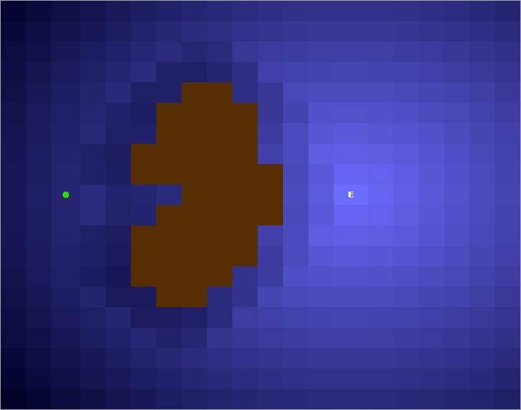
We solved this by using a trace similar to the pheromone trace described in [4]. Each agent controlling the unit adds a trace in the last N positions visited by the unit, as well as in the current position of the unit. The track generates a light repulsive potential and “pushes” the unit forward. See how the track pushes the unit around the local optimum (yellow line) and the unit can find the path to the destination.

But even with the traces, the risk remains that the unit will get stuck in situations like the one in the picture below.
This can be solved by filling in the voids:
Below, we criticized PP-based solutions from our point of view:
PP has problems like a local optimum that are difficult to solve. Using a trace, most local optima can be resolved. PP has problems in very difficult terrain; in these cases, methods of finding the way show themselves better. The power of PP is in handling large dynamic worlds with large open spaces and the least difficult terrain. This is the case for many of today's RTS games.
PP-based solutions require a lot of resources. In our work, we showed that PP-based solutions can be implemented with the same or even better efficiency as the path finding methods. Efficiency may be a problem, but in these cases path finding cases are more suitable.
PP-based solutions are difficult to implement and configure. PP can be implemented with a very simple architecture. Customization can be complicated and time-consuming, but the relative importance between the fields would be helpful here (for example, what is more important to destroy the base or units?). The graphical representation of PP is also very valuable.
Using Multi-agent Potential Fields in Real-time Strategy Games
Johan Hagelbäck and Stefan J. Johansson
International Conference on Autonomous Agents and Multi-agent Systems (AAMAS), 2008.
1. Download PDF
The Rise of Potential Fields in Real Time Strategy Bots
Johan Hagelbäck and Stefan J. Johansson.
Proceedings of Artificial Intelligence and Interactive Digital Entertainment (AIIDE), 2008.
2. Download PDF
A Multiagent Potential Field-Based Bot for Real-Time Strategy Games
Johan Hagelbäck and Stefan J. Johansson
International Journal of Computer Games Technology, 2009.
3. Download PDF
Learning Human-like Movement Behavior for Computer Games
C. Thurau, C. Bauckhage, and G. Sagerer
International Conference on the Simulation of Adaptive Behavior (SAB), 2004.
4. Download PDF
This lesson describes a game flow planning and unit navigation method that uses multi-agent potential fields. It is based on works under the numbers [1, 2, 3]. (See the end of the article for links to the materials used)
What is a potential field?
PP (Potential Field) has a number of similarities with influence maps. Influence cards are often used to determine whether a zone in the game world is under the control of a player or enemies (in the range of weapons or movement range), or is it a zone that is not currently controlled by anyone (no one’s land). The idea is to put positive values on the cells under the control of the player, and negative values under the control of the enemy. By smoothly decreasing the value to zero, we will create a map that reflects the influence of our and enemy units in the zone. The figure below shows an example of a map of influence with one of its own and one enemy unit.
Potential fields work in a similar way - a charge is put on an interesting position in the game world and generates a field that gradually goes to zero. The charge can be attractive (positive) or repulsive (negative). Note that in some literature on potential fields, negative charges are attractive and vice versa. In this lesson, positive charges are always hiding. The figure below shows a simple game world with some impassable territory (brown), an enemy unit (green) and the destination of the unit (E). The attracting charge is located at the destination.
The charge generates a field that spreads through the game world:
And fades to zero:
PP navigation
In the illustration above, the attractive field has spread around the destination point “E”. The point is to let the green unit move to the positions with the most attracted values and finally find the way to the destination. To make this work, we also need to deal with obstacles in the game world, in this case with mountains (cinnamon zones). If we force the mountains to generate small repulsive fields and add them to the attracting fields (from the figure above), we get a resulting field that can be used for navigation. Since units always move to a neighboring position with the most attractive value, we will go around the mountains if there is another way.
The same idea is used for other obstacles. In the picture below, two more of their units (white) were added. They generate small repulsive fields, which again add up to the resulting field.
Thus, our green unit will bypass these units to avoid a collision. Now we have got the final path for our unit. A unit can move from its current position to its destination and bypass all obstacles without using any algorithm for finding the path.
Benefits of Using PP
One of the main advantages of using potential fields is the ability to process dynamic game worlds. Since units (agents) move only one step at a time, instead of generating a full path from A to B, there is no risk that the path will become unavailable due to changes in the game world. Finding a path in a dynamic world can often be difficult to implement and require a lot of resources to calculate. When an approach based on potential fields is used, the solution to the problem comes automatically. Of course, you need to be careful when implementing the PP system, so as not to forget to make updating potential fields as effective as possible. (More about this later).
Another important advantage is the ability to create complex behavior by simply playing with the shape settings of the generated fields. Instead of linear attenuation to zero, we can use nonlinear fields. If, for example, we have shooting units like tanks in our army, we don’t want the tanks to move too close to the enemy units, but surround them at the right distance (for example, at the distance of their firing range). This behavior can be achieved by placing a zero charge at the location of the enemy unit, generating an increasing field with the most attracted point at the firing range, and then fading to zero. The picture below shows an example with two tanks (green) moving in an attack on an enemy unit (red), generating a non-linear PP.
An example of the equation of how such a field can be generated:
Here W1 is the value for changing the relative strength of the field. D is the maximum firing range and R is the maximum detection range (from where our agent sees the enemy agent).
Another behavior that is easy to implement is “kick-run”. First, the unit approaches the maximum attack distance.
After the attack, our unit must reload its weapon and retreats from the enemy unit until it is ready to shoot again.
During the retreat phase, all enemy units generate a strong repulsive field with a radius of the maximum range of the unit. This is an example of how specific potential fields can be active or inactive depending on the internal state of the agent controlling this unit. An inactive field is simply ignored when the resulting potential field is summed.
The image below is a screenshot of our software- based bot for ORTS.engine. The left side of the image is a 2D view of the current state of the game. It shows our tanks (green circles) going to attack enemy bases (red squares) and units (red circles). Brown and black zones - impassable territory (mountains). The potential field of this game state is shown on the right side of the image. As in other pictures from this lesson, the blue zones are the most attractive. The light lines are the attacks of our tanks. The PP view clearly shows how our units surround the enemy at the maximum range of the shot, while avoiding collisions with each other and the terrain. The behavior of the environment of the enemy works fine and was perhaps one of the key in our success of 2008 at the ORTS tournament.
While we were developing our bot for ORTS, we discovered one thing - a completely different behavior when summing the potentials of enemy units generated at each point was compared with simply the highest potential of the enemy unit at that point. In the figure below, the potentials generated by three enemy units are summed up and added to the resulting field. Thus, the greatest potential is directly in the center of the enemy unit cluster (circled in red) and our units were very keen to attack the enemies at their strongest points.
The solution was not to summarize the potentials, but instead to take the greatest potential at a point from all units. In the latter case, the highest potential around the enemies at an acceptable distance (shown by red lines).
Implementation Notes
With a good plan and implementation of the PP system, the cost of resources for calculation will not exceed traditional solutions based on the A * algorithm. Our ORTS bot used the least amount of CPU resources compared to two other bots working on path search algorithms since the 2007 tournament. However, we note that it is difficult to accurately calculate the CPU usage due to the fact that the winning bot uses more resources at the end of the game, as it has more units under control. Multithreading also complicates the task of calculating the required CPU resources. The comparison was carried out by comparing the total amount of CPU resources used by each client process in the Linux environment for 100 games. At least we can conclude that the bot was good within the allotted time of 0.125 seconds used in ORTS.
To improve performance, we divided software into three categories:
- Static fields. Fields that remain static throughout the game. In our case, the area. This field is generated at startup.
- Semi-static fields. Fields that do not require frequent updates. In our case, our and enemy bases. These fields are generated at startup and updated when the database is destroyed.
- Dynamic fields. All dynamic objects of the game world, such as ours and enemy tanks. These fields are updated every frame. To reduce the calculation time, you can count them every second or third frame.
We experimented with two main architectures for generating PP ...
Pre-generation
The field generated by each type of object was previously calculated and stored in static arrays in the header file. During the execution of the program, these fields were simply added to the general software at the desired position. To make this possible, the game world was divided into tiles, in our case, each tile consisted of 8x8 points of the game world. This approach showed insufficient detail and the bot performed poorly (2007 ORTS tournament). Since the game world was divided into significantly larger tiles, we ran into problems deciding which tile (which tiles) an object occupies. Assume an object (orange circle) and a base (orange square). What tiles (gray squares) does our green unit occupy and what tiles should the base occupy?
This approach may be suitable for games like Wargus, which use a less detailed tile navigation system.
Real-time calculations
The potentials generated at the point are calculated in real time by calculating the distance between the point and all nearby objects, passing each distance as a variable to a function and then calculating the potential. This approach, in fact, uses less CPU resources in our bot than pre-generated fields.
Thanks to:
- We consider the potentials of only those points that are candidates for the movement of units in them. In the pre-generated version, all potentials of the entire game world are considered (naturally, this can be optimized by a similar method).
- By calculating the distance to an object using the fast Manhattan method, we can avoid the costly calculation of distance in Euclidean space for a large number of objects in the game world.
This approach was used in the second version of our bot (2008 ORTS tournament). An example of the PP formula (with 2D and 3D graphs) used to calculate the potential generated by a cliff at a point with a distance “a” from the cliff.
And what about the problem of local optimum?
One of the most common problems with PP is the problem of local optimum. The picture below shows an example when this problem appears. Destination E generates a circular field that is blocked by the mountain. The unit moves to the positions with the highest potentials and finishes at the largest, where it currently stands. Unit stuck.
We solved this by using a trace similar to the pheromone trace described in [4]. Each agent controlling the unit adds a trace in the last N positions visited by the unit, as well as in the current position of the unit. The track generates a light repulsive potential and “pushes” the unit forward. See how the track pushes the unit around the local optimum (yellow line) and the unit can find the path to the destination.
But even with the traces, the risk remains that the unit will get stuck in situations like the one in the picture below.
This can be solved by filling in the voids:
Conclusion
Below, we criticized PP-based solutions from our point of view:
PP has problems like a local optimum that are difficult to solve. Using a trace, most local optima can be resolved. PP has problems in very difficult terrain; in these cases, methods of finding the way show themselves better. The power of PP is in handling large dynamic worlds with large open spaces and the least difficult terrain. This is the case for many of today's RTS games.
PP-based solutions require a lot of resources. In our work, we showed that PP-based solutions can be implemented with the same or even better efficiency as the path finding methods. Efficiency may be a problem, but in these cases path finding cases are more suitable.
PP-based solutions are difficult to implement and configure. PP can be implemented with a very simple architecture. Customization can be complicated and time-consuming, but the relative importance between the fields would be helpful here (for example, what is more important to destroy the base or units?). The graphical representation of PP is also very valuable.
References
Using Multi-agent Potential Fields in Real-time Strategy Games
Johan Hagelbäck and Stefan J. Johansson
International Conference on Autonomous Agents and Multi-agent Systems (AAMAS), 2008.
1. Download PDF
The Rise of Potential Fields in Real Time Strategy Bots
Johan Hagelbäck and Stefan J. Johansson.
Proceedings of Artificial Intelligence and Interactive Digital Entertainment (AIIDE), 2008.
2. Download PDF
A Multiagent Potential Field-Based Bot for Real-Time Strategy Games
Johan Hagelbäck and Stefan J. Johansson
International Journal of Computer Games Technology, 2009.
3. Download PDF
Learning Human-like Movement Behavior for Computer Games
C. Thurau, C. Bauckhage, and G. Sagerer
International Conference on the Simulation of Adaptive Behavior (SAB), 2004.
4. Download PDF