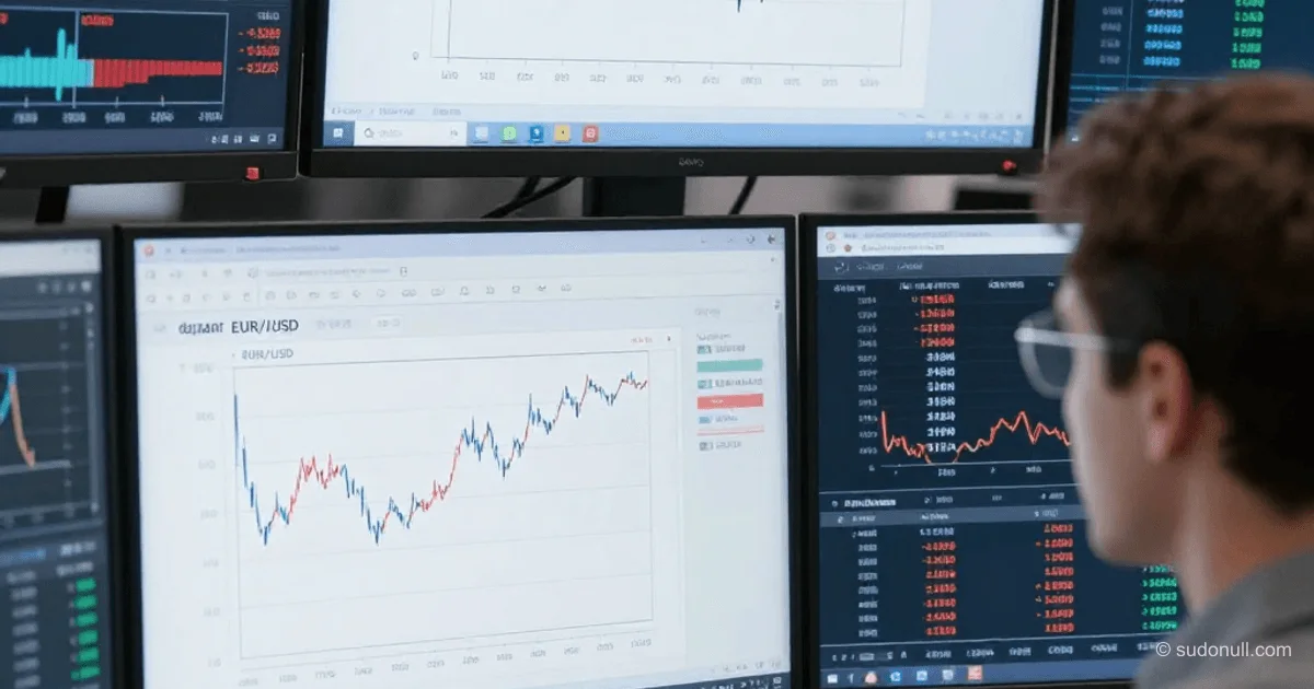
EURUSD volatility forecast in 4 lines of code

EUR/USD Volatility Forecast in 4 Lines: How dquant Simplifies ML for Traders Without Data Science

Modern algorithmic strategies demand precise, real-time risk assessment. Volatility is the key driver behind stop orders, position sizing, and capital management. Yet traditional approaches like GARCH and EWMA often fail to adapt to shifting market regimes, while ML solutions remain out of reach for most traders due to high barriers to entry—feature engineering, cross-validation, and hyperparameter tuning. The dquant library tackles this challenge at the API level: it encapsulates all preprocessing, training, and validation into just three method calls, eliminating the need to understand XGBoost’s inner architecture or manually craft features.

How VolClustXGB Works: From Raw OHLCV to Prediction

The VolClustXGB model is a specialized XGBoost regressor designed specifically for volatility forecasting. It doesn’t just predict price or direction—it outputs a scalar estimate of expected volatility (similar to an ATR-like metric) for a specified number of bars ahead. Under the hood, it implements a streamlined pipeline:

• Automatic generation of technical features from OHLCV data: True Range, logarithmic returns, absolute returns, price gaps, body-to-range ratio, shadow-to-body ratio, close-position relative to the range, and a 14-period rolling ATR (roll_atr_14).
• Splitting the time series into input windows (input_bars=70) and target values (horizon=20). The target variable is the volatility of the next 20 bars, calculated as the median or mean ATR over that horizon.
• Automated time-series-aware splitting of training and validation sets to prevent data leakage.
• Early stopping during training (early_stopping=True) based on declining validation error (RMSE or MAE), which prevents overfitting even with a large number of trees (trees_count=200).
• Visualization of the training process: a convergence plot showing error trends on both training and validation sets, allowing you to assess model stability.

All these steps are executed in a single .fit() call, without manual handling of indices, scaling, or data type conversions.

Practical Implementation: Code, Interpretation, and Limitations

The reference example uses hourly EUR/USD data from Yahoo Finance. It’s crucial to recognize that the data source directly impacts forecast quality: yfinance limits intraday data to 730 days, which may not be sufficient for training on diverse market cycles—from low volatility periods to spikes caused by FOMC meetings or geopolitical events. An alternative is MetaTrader 5, which provides access to longer histories (up to 1,000+ days) via the local terminal and broker account.

Key parameters for the .fit() call include:

• feature_list: a list of features that will be automatically computed. By default, it uses a set optimized for currency pairs, but you can expand or replace it.
• input_bars: the length of the input window. A value of 70 corresponds to roughly three days on an hourly timeframe—enough to capture short-term volatility patterns.
• horizon: the forecast horizon. For hourly data, horizon=20 means a 20-hour forecast, useful for intraday risk-management strategies.
• show_results: displays the training graph. Recommended for development use to diagnose overfitting.

After training, the forecast is generated with a .forecast() call using the same number of bars as input_bars. The result is an array of predicted volatility values compatible with any risk-management module.

Key Takeaways

• No need to manually create features: the library automatically generates TR, returns, roll_atr_14, and other technical metrics from OHLCV.
• Time-series robustness: the built-in time-series split ensures validation data always lies in the future relative to training data.
• Early stopping by default: training halts when validation error starts rising, regardless of the specified trees_count.
• Persistence and reusability: the model can be saved in serialized form via .save() and loaded via .load(), enabling production use without retraining.
• Open MIT license: the code is available for auditing, modification, and integration into proprietary systems without legal restrictions.

Integrating into a Trader’s Workflow

For practical application, we recommend the following pipeline:

• Daily updates of historical data via MT5 (or yfinance if 730 days suffice).
• Recalculating the volatility forecast for the next 20 bars before opening each trading session.
• Using the forecasted value to dynamically calibrate stop-losses—for example, stop_distance = forecasted_volatility * 1.5.
• Saving the model after each successful training run and comparing its performance against previous versions using RMSE on out-of-sample test data.

Note that dquant is not a full-fledged trading platform. It’s a tool for generating risk signals. Its outputs should be integrated into existing strategies through standard interfaces (pandas DataFrames, numpy arrays). Direct integration with MT5 is possible via mt5.order_send(), using the forecasted value as an input parameter for volume calculation.

— Editorial Team