Gradient Descent and Backpropagation in Neural Networks: CUDA/C++

Gradient Descent & Backpropagation: Training Neural Networks from Scratch with CUDA/C++

This article is the fourth part of a deep dive into the world of neural networks, where we are building a Transformer architecture step-by-step, starting with the most basic components in CUDA. In this installment, we move from implementing the forward pass to the crucial stage of model training. We will explore the fundamental mechanisms of Gradient Descent and Backpropagation, implementing them at a low level using C++ and CUDA to train our neural network to recognize handwritten digits from the MNIST dataset. The goal is not just to use off-the-shelf libraries, but to thoroughly understand how these complex computational processes work "under the hood," which is critical for a deep comprehension of modern machine learning and artificial intelligence models.

Fundamentals of Neural Network Training: Gradient Descent

After successfully implementing the forward pass in the previous part, our model is capable of making predictions. However, at the initial stage, without training, these predictions will be random. For the model to start producing correct results, its internal parameters (weights and biases) must be adjusted to minimize the error between predictions and true labels. Algorithms like Gradient Descent and Backpropagation are used precisely for this purpose.

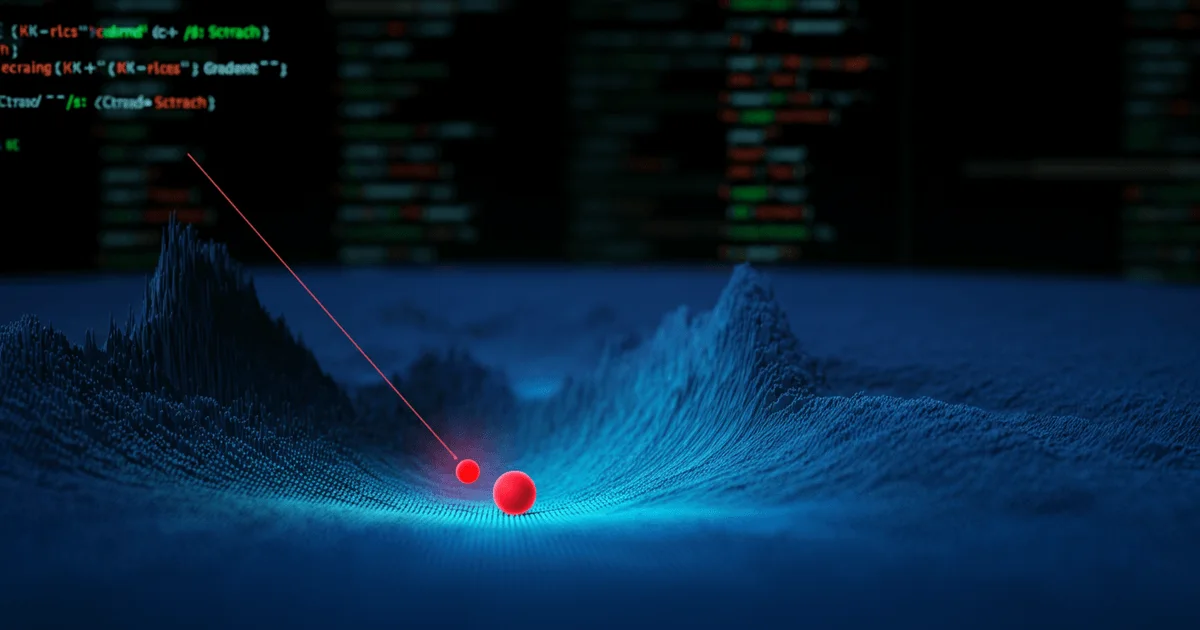
Imagine you are on a mountaintop in a dense fog, and your task is to descend to the lowest point of the valley. You cannot see the entire landscape, but you can feel the slope under your feet. The gradient is a vector that indicates the direction of the steepest ascent. Consequently, to descend, you need to move in the opposite direction of the gradient. In the context of neural networks, the "mountain" is the surface of the error function (or loss function), and the "valley" is its global minimum. The goal of gradient descent is to find this minimum by iteratively adjusting the network's weights in the direction opposite to the gradient of the loss function with respect to these weights.

Backpropagation is an algorithm that efficiently computes these gradients. It works by propagating the error from the network's output layer back to the input layer, distributing responsibility for the error among all weights. Mathematically, this is implemented through the Chain Rule of differentiation, which allows us to calculate how a change in each weight affects the model's overall error.

Loss Function: Cross-Entropy

To measure the "badness" of the model's predictions, a loss function is used. In classification tasks, such as recognizing handwritten MNIST digits, cross-entropy loss is a standard choice. It quantifies the divergence between the probability distribution predicted by the model and the true distribution (where only the correct class has a probability of 1, and others are 0). The greater this divergence, the higher the loss function value.

For a single example, cross-entropy is calculated using the formula:

![L = -\sum_{i=1}^{K} y_i \log(\hat{y}_i)](./images/image-1.svg)

Where:

![K](./images/image-2.svg) — is the number of classes (for MNIST, this is 10).
![y_i](./images/image-3.svg) — is the true value (1 for the correct class, 0 for others).
![\hat{y}_i](./images/image-4.svg) — is the model's prediction (probability obtained after the Softmax layer).

Since training usually occurs on batches of data, not individual examples, the total loss function for a batch is averaged over its size (![N](./images/image-5.svg) — batch size):

![L = -\frac{1}{N} \sum_{j=1}^{N} \sum_{i=1}^{K} y_{j,i} \log(\hat{y}_{j,i})](./images/image-6.svg)

Below is the C++ code for calculating cross-entropy on the CPU, which simplifies debugging and understanding:

float cross_entropy_loss_cpu(
  const Tensor& predictions, const std::vector<int>& labels
) {
  int batch_size = predictions.shape()[0];
  int num_classes = predictions.shape()[1];
  float loss = 0.0f;
  for (int i = 0; i < batch_size; i++) {
    for (int j = 0; j < num_classes; j++) {
      float prob = predictions.get({i, j});
      float target = (labels[i] == j) ? 1.0f : 0.0f;
      loss += -std::log(prob) * target;
    }
  }
  return loss / batch_size;
}

Backpropagation and the Chain Rule

To minimize the loss function ![L](./images/image-9.svg), we need to know how its value changes with a small change in each weight in the network. This is the gradient of the loss function with respect to the weights. For example, for weight ![W_1](./images/image-10.svg) of the first layer, we need to find ![\frac{\partial L}{\partial W_1}](./images/image-8.svg).

The architecture of our network, developed in previous articles, looks as follows:

First Linear Layer: ![z_1 = W_1 \cdot x + b_1](./images/image-11.svg)
Activation (ReLU): ![a_1 = \sigma(z_1)](./images/image-12.svg)
Second Linear Layer: ![z_2 = W_2 \cdot a_1 + b_2](./images/image-13.svg)
Output (Softmax + Loss): ![L = Loss(Softmax(z_2))](./images/image-14.svg)

To calculate the gradient ![\frac{\partial L}{\partial W_1}](./images/image-16.svg), we apply the Chain Rule:

![\frac{\partial L}{\partial W_1} = \frac{\partial L}{\partial z_2} \cdot \frac{\partial z_2}{\partial a_1} \cdot \frac{\partial a_1}{\partial z_1} \cdot \frac{\partial z_1}{\partial W_1}](./images/image-17.svg)

Each term in this chain represents a local gradient, which shows how the output of a given layer or function affects its input. Backpropagation begins by calculating the gradient of the loss function with respect to the outputs of the last layer, and then sequentially propagates this gradient backward through all layers of the network.

Detailed Derivation of Gradients for Softmax and Cross-Entropy

Let's start from the very end of the chain – the derivative of the loss function ![L](./images/image-25.svg) with respect to the outputs of the second linear layer ![z_2](./images/image-20.svg) after applying Softmax. This is one of the most important and frequently used gradients. Recall how Softmax looks for each element ![i](./images/image-19.svg) in the vector ![z_2](./images/image-20.svg):

![a_{2, i} = \frac{e^{z_i}}{\sum_{j=1}^{K} e^{z_j}}](./images/image-21.svg)

Where ![z_2](./images/image-22.svg) is the output of the second linear layer (logits), and ![a_2](./images/image-23.svg) is the result of Softmax (probabilities). The gradient ![\frac{\partial L}{\partial z_{2,i}}](./images/image-18.svg) can be decomposed using the Chain Rule:

![\frac{\partial L}{\partial z_{2,i}} = \sum_{k=1}^{K} \frac{\partial L}{\partial a_{2,k}} \cdot \frac{\partial a_{2, k}}{\partial z_{2,i}}](./images/image-24.svg)

First, let's find the derivative of the loss function ![L](./images/image-27.svg) with respect to ![a_i](./images/image-26.svg):

![\frac{\partial L}{\partial a_i} = \frac{\partial}{\partial a_i} \left( -y_i \ln(a_i) \right) = -y_i \cdot \frac{1}{a_i} = -\frac{y_i}{a_i}](./images/image-29.svg)

Now let's move to the derivative of Softmax with respect to ![z](./images/image-30.svg). Here, the quotient rule for differentiation will be needed. The Softmax formula: ![a_i = \frac{e^{z_i}}{\sum_{k=1}^K e^{z_k}}](./images/image-32.svg)

If ![i=j](./images/image-43.svg), the derivative is:

![\frac{\partial a_i}{\partial z_i} = a_i (1 - a_i)](./images/image-36.svg)

If ![i \neq j](./images/image-37.svg), the derivative is:

![\frac{\partial a_i}{\partial z_j} = -a_i a_j](./images/image-41.svg)

Using the Kronecker delta symbol ![\delta_{ij}](./images/image-42.svg), these two cases can be combined:

![\frac{\partial a_i}{\partial z_j} = a_i (\delta_{ij} - a_j)](./images/image-44.svg)

Combining the derivatives of cross-entropy and Softmax, we get:

![\frac{\partial L}{\partial z_i} = \sum_{k=1}^{K} \left( -\frac{y_k}{a_k} \right) \cdot \left( a_k(\delta_{ki} - a_i) \right) = \sum_{k=1}^{K} -y_k (\delta_{ki} - a_i)](./images/image-49.svg)

Further simplification, considering that the sum of true probabilities ![\sum_{k=1}^{K} y_k](./images/image-51.svg) is always equal to 1, leads to a surprisingly simple and elegant formula:

![\frac{\partial L}{\partial z_i} = a_i - y_i](./images/image-52.svg)

This means that the gradient of the loss function with respect to the logits (outputs before Softmax) is simply the difference between the predicted probabilities and the true labels. This result is a cornerstone for implementing backpropagation in classification models.

Implementing the Gradient in C++

Applying the derived formula, we can implement the gradient calculation for the last layer of our neural network. This gradient will then be used to update the weights, moving the model towards a smaller error. Here's how it looks in C++ code:

auto grad = Tensor::create_zeros({ batch_size, num_classes });

for (int i = 0; i < batch_size; ++i) {
  for (int j = 0; j < num_classes; ++j) {
    float prob = fc2.output->get({i, j});
    float target = (targets[i] == j) ? 1.0f : 0.0f;
    float gradient = (prob - target) / batch_size; // Division by batch_size for averaging
    grad->set({i, j}, gradient);
  }
}

This code calculates the error gradient for each element in the batch and then averages it over the batch size. The resulting grad tensor contains information on how much to change the logits ![z_2](./images/image-54.svg) to reduce the error. This gradient will then be propagated through the preceding layers of the network, allowing the weights ![W_2](./images/image-13.svg), ![b_2](./images/image-13.svg), ![W_1](./images/image-11.svg), and ![b_1](./images/image-11.svg) to be adjusted using the corresponding local derivatives.

Key Takeaways:

Gradient Descent is an iterative optimization method that adjusts model parameters in the direction opposite to the gradient of the loss function to find its minimum.
Backpropagation is an algorithm that uses the chain rule to efficiently compute the gradients of the loss function with respect to all weights in a neural network.
Cross-Entropy is a standard loss function for classification tasks, measuring the divergence between predicted and true probability distributions.
The derivative of Softmax + Cross-Entropy with respect to logits simplifies to the difference between predicted probabilities and true labels, significantly simplifying implementation.
Implementing from scratch in C++/CUDA allows for a deep understanding of the internal mechanisms of models like Transformer, without relying on high-level abstractions.

— Editorial Team