Ethernet Channel Bandwidth Measurement
There was a task to measure the bandwidth of the Ethernet channel and provide a report, and the measurements need to be done 24 hours. How can this be done?
Using the iperf tool is very simple: on one side of the channel, a server starts on the computer and waits for a connection from the client:
On the other side of the channel, on a different computer, a client starts up with an ip server:
As you can see from the report, the throughput was measured for 10 seconds and amounted to 28.2 Gbit / s (the speed is so high because both the server and the client were running on the same computer). Great, but we need to measure speed for a whole day. We look at the iperf --help options and find a bunch of useful information there. As a result, I got something like this:
The -t 86400 parameter sets the measurement time in seconds, and the -i 15 parameter tells you to output a result every 15 seconds. It’s already better, but not very convenient, to view such a report for a whole day (in such a report there will be 86400/15 = 5760 lines). We look at help further and see that iperf can provide a report in the form:
We check:
Excellent! Exactly what is needed! Now iperf provides statistics convenient for processing. Parameters in the report are separated by commas. The first column is the date and time, then the IP addresses and ports of the client and server are visible, at the end, the bandwidth in bits / s. Redirect this report to a file:
After the end of the daily test, the stat.txt file neatly contains the results that need to be visualized in a convenient form for analysis.
So, the stat.txt file contains the results of the channel throughput tests for the right time with a given interval. Of course, you can look through each of several thousand lines with your eyes and do the analysis, but once people came up with computers, first of all, to facilitate their work, and not to look at cats in contact people, and we will use this invention.
The report file contains data necessary and not very. Get rid of the extra. We are interested in the date / time of the measurement and the speed at that date / time. This is the first and last parameter in each line of the stat.txt file.
I processed this file hastily with a written script in python3, please do not judge for the curvature of the code - I am a fake welder, I found a mask at a construction site.
This script reads the lines from the stat.txt file and writes the results to the est.txt file. In the est.txt file it turns out:
Already more convenient. Shows the date, time, the measurement result in Mbps. For this example, the measurement results for 10 minutes are taken with a report every second.
But still the result in the form of a text file is not very convenient for analysis. We need to draw a chart!
There are special and cool programs for drawing graphs. I advise gnuplot for its super flexibility, free of charge, a bunch of examples on the Internet.
After half an hour of digging in the results of Google’s query “gnuplot example”, I got the following script:
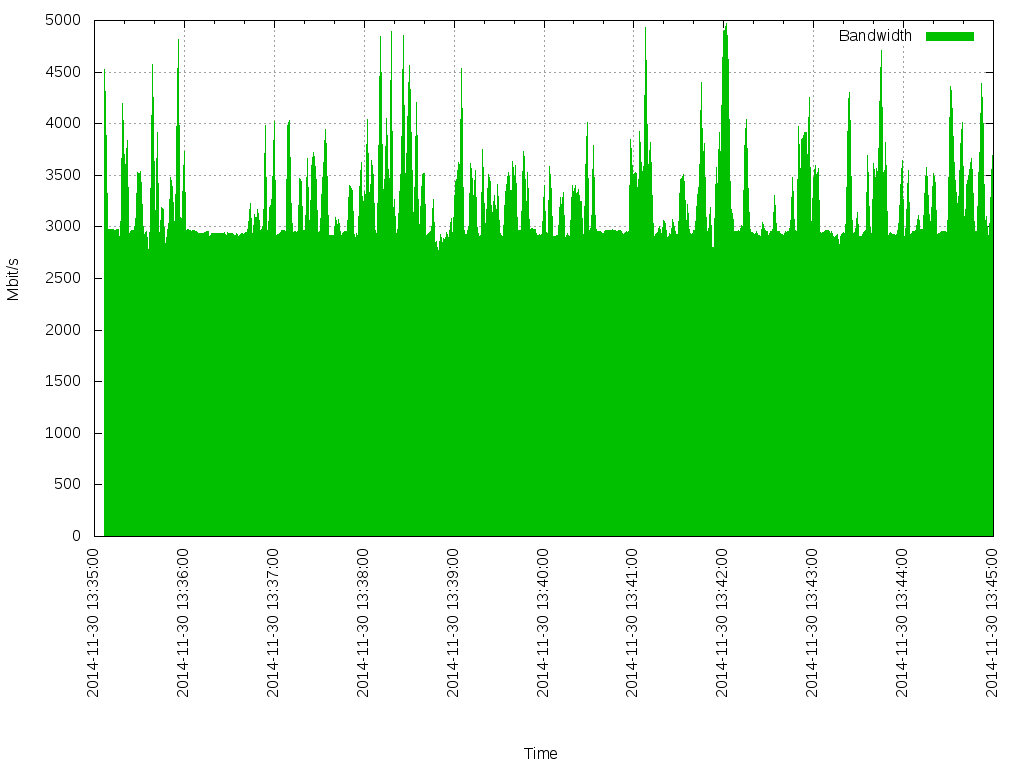
This script reads the est.txt file that came after processing stat.txt and draws the graph into the graph.png file. We start and the graph.png file appears.
As a result, a simple technique for measuring channel bandwidth with a visually convenient report and two data processing scripts appeared.
In these scripts, you can cram a bunch of other things for flexibility, such as: a report for a given time interval, more detailed chart detail for closer inspection, fasten ping response time analysis, along with collecting daily data, remove other data such as signal levels from channel-forming equipment via SNMP on the radio channel and BER indicators, but that's another story.
Than
- Service speedtest.net - measures the width of the Internet channel to a server. It doesn’t suit us because this service measures not a specific communication channel, but the entire line to a specific server; the measured communication channel also does not have Internet access;
- Download a volume file from one end of the channel to the other. Not quite suitable as there is no necessary measurement accuracy;
- Iperf is a client-server utility that allows you to measure a given time with the provision of a simple report. We’ll work with her now.
how
Using the iperf tool is very simple: on one side of the channel, a server starts on the computer and waits for a connection from the client:
d@i:~$ iperf -s
------------------------------------------------------------
Server listening on TCP port 5001
TCP window size: 85.3 KByte (default)
------------------------------------------------------------
On the other side of the channel, on a different computer, a client starts up with an ip server:
d@i:~$ iperf -c 172.28.0.103
------------------------------------------------------------
Client connecting to 172.28.0.103, TCP port 5001
TCP window size: 2.50 MByte (default)
------------------------------------------------------------
[  3] local 172.28.0.103 port 56868 connected with 172.28.0.103 port 5001
[ ID] Interval       Transfer     Bandwidth
[  3]  0.0-10.0 sec  32.9 GBytes  28.2 Gbits/sec
As you can see from the report, the throughput was measured for 10 seconds and amounted to 28.2 Gbit / s (the speed is so high because both the server and the client were running on the same computer). Great, but we need to measure speed for a whole day. We look at the iperf --help options and find a bunch of useful information there. As a result, I got something like this:
d@i:~$ iperf -c 172.28.0.103 -t 86400 -i 15
------------------------------------------------------------
Client connecting to 172.28.0.103, TCP port 5001
TCP window size: 2.50 MByte (default)
------------------------------------------------------------
[  3] local 172.28.0.103 port 56965 connected with 172.28.0.103 port 5001
[ ID] Interval       Transfer     Bandwidth
[  3]  0.0-15.0 sec  58.0 GBytes  33.2 Gbits/sec
[  3] 15.0-30.0 sec  50.4 GBytes  28.9 Gbits/sec
[  3] 30.0-45.0 sec  47.4 GBytes  27.2 Gbits/sec
[  3] 45.0-60.0 sec  51.8 GBytes  29.7 Gbits/sec
[  3] 60.0-75.0 sec  45.5 GBytes  26.1 Gbits/sec
[  3] 75.0-90.0 sec  43.2 GBytes  24.7 Gbits/sec
[  3] 90.0-105.0 sec  54.6 GBytes  31.3 Gbits/sec
The -t 86400 parameter sets the measurement time in seconds, and the -i 15 parameter tells you to output a result every 15 seconds. It’s already better, but not very convenient, to view such a report for a whole day (in such a report there will be 86400/15 = 5760 lines). We look at help further and see that iperf can provide a report in the form:
-y, --reportstyle C report as a Comma-Separated Values
We check:
d@i:~$ iperf -c 172.28.0.103 -t 86400 -i 15 -y C
20141130132436,172.28.0.103,56976,172.28.0.103,5001,3,0.0-15.0,59595292672,31784156091
20141130132451,172.28.0.103,56976,172.28.0.103,5001,3,15.0-30.0,49530142720,26416076117
20141130132506,172.28.0.103,56976,172.28.0.103,5001,3,30.0-45.0,57119866880,30463929002
Excellent! Exactly what is needed! Now iperf provides statistics convenient for processing. Parameters in the report are separated by commas. The first column is the date and time, then the IP addresses and ports of the client and server are visible, at the end, the bandwidth in bits / s. Redirect this report to a file:
d@i:~$ iperf -c 172.28.0.103 -t 86400 -i 15 -y C > stat.txt
After the end of the daily test, the stat.txt file neatly contains the results that need to be visualized in a convenient form for analysis.
And now what to do with it?
So, the stat.txt file contains the results of the channel throughput tests for the right time with a given interval. Of course, you can look through each of several thousand lines with your eyes and do the analysis, but once people came up with computers, first of all, to facilitate their work, and not to look at cats in contact people, and we will use this invention.
The report file contains data necessary and not very. Get rid of the extra. We are interested in the date / time of the measurement and the speed at that date / time. This is the first and last parameter in each line of the stat.txt file.
I processed this file hastily with a written script in python3, please do not judge for the curvature of the code - I am a fake welder, I found a mask at a construction site.
#!/usr/bin/env python3
import datetime
st = open('stat.txt', 'r')
res = open('est.txt', 'w')
for line in st:
    w = line.split(',')
    ti = datetime.time(int(w[0][-6:][0:2]), int(w[0][-6:][2:4]), int(w[0][-6:][4:6]))
    da = datetime.date(int(w[0][0:8][0:4]), int(w[0][0:8][4:6]), int(w[0][0:8][6:9]))
    print("{0} {1} {2}".format(da, ti, int(w[8])/(1024**2)), file=res)
res.close()
This script reads the lines from the stat.txt file and writes the results to the est.txt file. In the est.txt file it turns out:
 d@i:~/project/iperf_graph$ cat est.txt
2014-11-30 13:35:07 4521.25
2014-11-30 13:35:08 3682.875
2014-11-30 13:35:09 2974.75
2014-11-30 13:35:10 2974.625
2014-11-30 13:35:11 2976.375
2014-11-30 13:35:12 2976.25
2014-11-30 13:35:13 2977.0
2014-11-30 13:35:14 2969.75
Already more convenient. Shows the date, time, the measurement result in Mbps. For this example, the measurement results for 10 minutes are taken with a report every second.
But still the result in the form of a text file is not very convenient for analysis. We need to draw a chart!
There are special and cool programs for drawing graphs. I advise gnuplot for its super flexibility, free of charge, a bunch of examples on the Internet.
After half an hour of digging in the results of Google’s query “gnuplot example”, I got the following script:
#! /usr/bin/gnuplot -persist
set term png size 1024,768
#set terminal postscript eps enhanced color size 1024, 768
set output "graph.png"
set grid
set yrange[0:]
set xdata time
set xlabel "Time"
set ylabel "Mbit/s"
set timefmt "%Y-%m-%d %H:%M:%S"
set format x "%Y-%m-%d %H:%M:%S"
set xrange [] noreverse nowriteback
set xtics rotate
plot "est.txt" using 1:3 title "Bandwith"  with filledcurve x1 lt 1 lc 2
This script reads the est.txt file that came after processing stat.txt and draws the graph into the graph.png file. We start and the graph.png file appears.
Result
As a result, a simple technique for measuring channel bandwidth with a visually convenient report and two data processing scripts appeared.
In these scripts, you can cram a bunch of other things for flexibility, such as: a report for a given time interval, more detailed chart detail for closer inspection, fasten ping response time analysis, along with collecting daily data, remove other data such as signal levels from channel-forming equipment via SNMP on the radio channel and BER indicators, but that's another story.