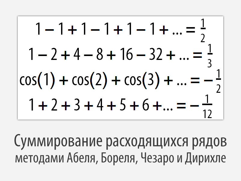
Summation of divergent series by the methods of Abel, Borel, Cesaro and Dirichlet

Translation of Devendra Kapadia's post " The ABCD of Divergent Series ."
I express gratitude to the help in the translation to Andrey Dudin .

What is the sum of all natural numbers? Intuition tells us that the answer is infinity. In mathematical analysis, the sum of natural numbers is a simple example of a divergent series. Nevertheless, mathematicians and physicists have found it useful to give fractional, negative, and even zero values ​​to the sums of such series. The purpose of my article is the desire to move the veil of secrecy surrounding the results of summing up divergent series. In particular, I will use the Sum function (the function of searching for partial sums, series, etc. in Mathematica), as well as other functions in Wolfram Language in order to explain in what sense it is worth considering the following statements:



The importance of the notation of formulas with the letters A, B, C, and D will soon become clear to you.

To begin with, we recall the concept of a convergent series using the following infinitely decreasing geometric progression.



The general term of the series, starting from n = 0 , is determined by the formula:

In [1]: =



Now we define the sum of the terms of the series from i = 0 to some finite value i = n .

In [2]: =



This finite sum is called the partial sum of the series .

The graph of the values ​​of such partial sums shows that their values ​​approach the number 2 with increasing n :

In [3]: =



Out [3] =



Using the Limit function (searching for the limit of a sequence or function at a point) we find the limit of the value of the partial sums of this series as nto infinity, which confirms our observations.

In [4]: ​​=



Out [4] =



The Sum function gives the same result when we sum the members of the series from 0 to infinity.

In [5]: =



Out [5] =



We say that a given series (the sum of a given infinitely decreasing geometric progression) converges and that its sum is 2.

In general, an infinite series converges if the sequence of its partial sums tends to a certain value for unbounded increasing the number of the partial amount. In this case, the limit value of the partial sums is called the sum of the series.

An infinite series that does not converge is called divergent. By definition, the sum of a divergent series cannot be found using the partial sum method discussed above. However, mathematicians have developed various ways of assigning finite numerical values ​​to the sums of these series. This amount is called the regularized sum of the divergent series. The process of calculating regularized sums is called regularization .



Now we look at example A from the introduction.



“A” stands for Abel, the famous Norwegian mathematician who proposed one of the techniques for regularizing divergent series. During his short life, he died at only 26 years old, Abel achieved impressive results in solving some of the most difficult mathematical problems. In particular, he showed that a solution to a fifth-degree algebraic equation cannot be found in radicals, thereby putting an end to a problem that remained unresolved for 250 years before it.

In order to apply the Abel method, we note that the general term of this series has the form:

In [6]: =



This can be easily checked by finding the first few values ​​of a [ n ].

In [7]: =



Out [7] =



As can be seen in the graph below, the partial sums of the series take values ​​equal to 1 or 0, depending on whether even n or odd.

In [8]: =



Out [8] =



Naturally, the Sum function displays a message that the series is diverging.

In [9]: =





Out [9] =



Abel's regularization can be applied to this series in two steps. First, we construct the corresponding power series.

In [10]: =



Out [10] =



Then we take the limit of this sum for x tending to 1, and note that the corresponding series converges for x values smaller but not equal to 1.

In [11]: =



Out [11 ] =



These two steps can be combined, forming, in essence, the definition of the sum of the divergent series according to Abel .

In [12]: =



Out [12] =



We can get the same answer using the Regularization option for the Sum function as follows.

In [13]: =



Out [13] =



Value 1 / 2 seems reasonable, because it is the average value of two values, 1 and 0, the partial sum of the received series. In addition, the limit transition used in this method is intuitive, since at x= 1 power series coincides with our divergent series. However, Abel was greatly concerned about the lack of rigor inherent in the mathematical analysis of the time, and expressed his concern about this:

“The diverging ranks are the devil’s invention, and it’s embarrassing to refer to them for any evidence. With their help, you can draw any conclusion that suits him, and that is why these series produce so many mistakes and so many paradoxes. ” (N.H. Abel in a letter to his former teacher Berndt Holmboy, January 1826)



We now turn to example B, which states that:



“B” stands for Borel, a French mathematician who worked in areas such as measure theory and probability theory. In particular, Borel is associated with the so-called “endless monkey theorem,” which states that if an abstract monkey randomly hits the typewriter’s keyboard for an infinite amount of time, then it’s likely that it will print some specific text, for example, a complete collection of works by William Shakespeare, nonzero.

In order to apply the Borel method, we note that the general term of this series has the form:

In [14]: = The



Borel regularization can be applied to rapidly diverging series in two steps. In the first step, we calculate the exponential generating functionfor a sequence of members of a given series. The factorial in the denominator ensures the convergence of this series for all values ​​of the parameter t .

In [15]: =



Out [15] =



Then we perform the Laplace transform of our exponential generating function and look for its value at the point s = 1 .

In [16]: =



Out [16] =



Out [17] =



These steps can be combined, as a result we get, in essence, the definition of the sum of the divergent series according to Borel .

In [18]: =



Out [18] =



We can also use specialized Wolfram Language functions to search for an exponential generating function and the Laplace transform:

In [19]: =



Out [19] =



Moreover, the answer can be obtained directly using Sum as follows.

In [20]: =



Out [20] =



The determination of the sum by Borel is reasonable, because it gives the same result as the usual method of partial sums, if applied to a convergent series. In this case, we can swap the summation and integration, and then determine the Gamma function , and we get that the corresponding integral will be equal to 1 and it will remain simple, in fact, the initial sum of the series:

In [21]: =



Out [21] =



However, in the case of divergent rows, the signs of the sum and the integral cannot be interchanged, which leads to interesting results that this regularization method gives.

Borel summation is a universal method of summing divergent series, which is used, say, in quantum field theory. There is a huge collection of literature on the application of Borel summation.



Example C states that:



“C” stands for Cesaro (in English his last name is spelled Cesaro), an Italian mathematician who made a significant contribution to differential geometry, number theory, and mathematical physics. Cesaro was a very productive mathematician and wrote about 80 works between 1884 and 1886, before he received his PhD in 1887!

To begin with, we note that the general term of the series, starting with n = 0, has the form:

In [22]: = The



graph shows a strong oscillation of the partial sums of this series.

In [23]: =



Out [23] =



The Cesaro method uses a sequence of arithmetic means of the partial sums of a series in order to suppress the oscillations, as shown in the following graph.

In [24]: =



Out [24] =



Formally speaking, Cesaro summation is defined as the limit of a sequence of arithmetic mean values ​​of partial sums of a series. Calculating this limit for the series from Example C, we get the result we expected -1/2 (see the graph above).

In [25]: =



Out [25] =



The Cesaro sum can be obtained directly if we use this type of regularization in the Sum function by specifying the appropriate value for the Regularization option.

In [26]: =



Out [26] =



The Cesaro summation method plays an important role in the theory of Fourier seriesin which series based on trigonometric functions are used to represent periodic functions. The Fourier series for a continuous function may not converge, but the corresponding Cesaro sum (or Cesaro mean, as it is usually called) will always converge to the function. This beautiful result is called the Fejér theorem.



Our last example claims that the sum of the natural series is -1/12.



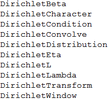
“D” means Dirichlet, a German mathematician who made a huge contribution to number theory and several other areas of mathematics. The breadth of Dirichlet's contributions can be judged by simply entering the following code in Mathematica 10.

In [27]: =



Out [27] // TableForm =



Dirichlet regularization got its name from the concept of “Dirichlet series”, which is defined as follows:



A special case of this series is the Riemann zeta function , which can be defined as follows:

In [28 ]: =



In [29]: =



Out [29] =



The SumConvergence function tells us that this series converges if the real part of the parameter s is greater than 1.

In [30]: =



Out [30] =



However, the Riemann zeta function itself can also be determined for other values ​​of the parameter s using the process of analytic continuation, known from the theory of functions of a complex variable. For example, for s = -1, we get:

In [31]: =



Out [31] =



But for s = -1, the series defining the Riemann zeta function is a natural series. From here we get that:

In [32]: =



Out [32] =



Another way of recognizing this result is to introduce an infinitesimal parameter ε into the expression of a member of our divergent series, and then find the expansion of the resulting function in the Maclaurin series using the Series function as shown below.

In [33]: =



Out [33] =



The first term in the expansion above tends to infinity as the parameter ε approaches zero, at the same time, the third term and all the following terms tend to zero. If we discard all terms depending on ε, then the remaining number -1/12 will be the Dirichlet sum of the natural series. Thus, the Dirichlet sum is obtained by discarding the infinitesimal and infinitely large terms of the expansion of the series constructed by the method described by us. This contradicts the fact that it is customary to discard only infinitesimal quantities in ordinary mathematical analysis; therefore, the result of summing divergent Dirichlet series is not so intuitive.

Similarly, you can get an incredibly strange value of 0 for a diverging sum of squares of natural numbers.

In [34]: =



Out [34] =



In this case, the corresponding expansion does not contain terms independent of the parameter ε, as a result we get 0.

In [35]: =



Out [35] =





Dirichlet regularization is closely related to the zeta regularization process, which is used in modern theoretical physics. In his famous work, the outstanding British physicist Stephen Hawking applied this method to the problem of calculating Feynman integrals in curved space-time. Hawking's article describes the zeta-regularization process very systematically and has gained great popularity since publication.

Our knowledge of divergent series is based on the most profound theories developed by some of the best thinkers of the last few centuries. However, I agree with many readers who, like me, feel some misunderstanding when they see them in modern physical theories. The great Abel was probably right when he called these series "the invention of the devil." It is possible that some future Einstein, who has a mind free from all sorts of foundations and authorities, will discard the prevailing scientific beliefs and reformulate fundamental physics so that there is no room for diverging series. But even if such a theory becomes a reality, divergent series will still give us a rich source of mathematical ideas, illuminating the path to a deeper understanding of our universe.