Video Processing Algorithms on TI DM368 Processor
We begin a series of articles on Habré dedicated to the TI DM368, DM369 video processors and the development of algorithms based on them.
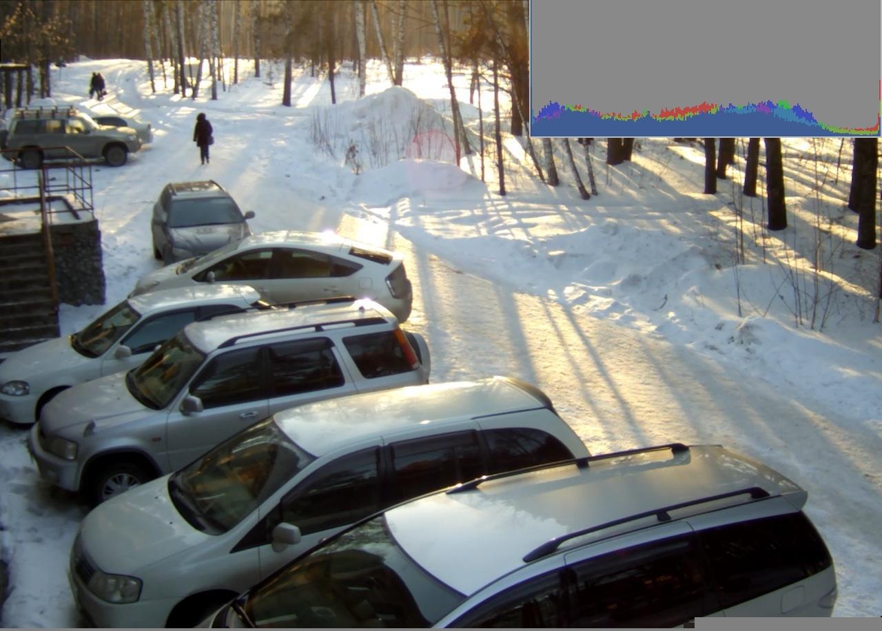
Let us examine the main blocks of video stream processing from the sensor to the network “broadcaster”, we will dwell in more detail on the algorithms of autoexposure, white balance and autofocus (3A), gamma correction, as well as the extended dynamic range of HDR or WDR, and finally, motion detection and analytics on its basis.
Examples of pictures will be presented for the SONY IMX136 sensor , the algorithm is also tested on Aptina MT9P006 , AR0331 , MT9M034 sensors .
The main players in the processor market for ip video surveillance are 3 companies TI , Ambarella and Hisilicon . All of them have chips of different price ranges, the most popular on the market right now with the ability to encode FHD (1920x1080) video stream up to 30 frames per second DM368 (TI), A5 (Ambarella), Hi3516 (Hisilicon) at a price of $ 10 to $ 20 and more powerful up to 60 frames per second DM385 (TI), A7 (Ambarella), Hi3517 (Hisilicon) at a price of $ 20 to $ 40. The characteristics of these chips are approximately the same.
Since TI is a fairly open company, all the hardware documentation is on the site, it is easiest to work with. To get the software and the whole design, just buy a camera from Approfor $ 1,000 and more. To obtain documentation from HiSilicon, you must sign an NDA, and the cost of support and a reference fee is $ 5,000. The most expensive was Ambarella, to get the documentation and support you need to shell out $ 25,400.
So, back to DM368:
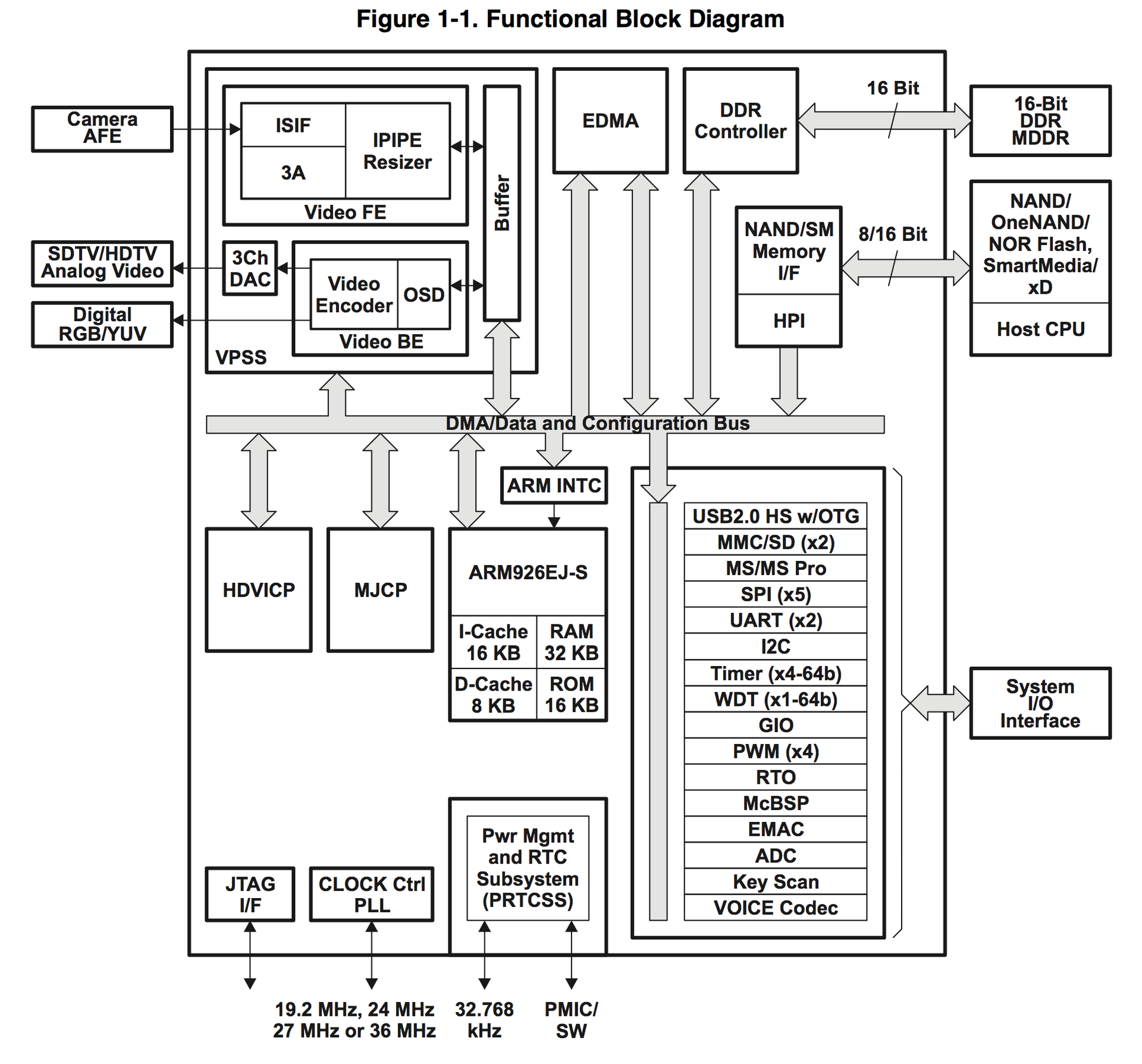
As you can see in the diagram, the processor has everything that is needed for the ip camera and not only for it. Video Processing Subsystem (VPSS) is involved in video processing; in turn, it consists of two Video FE (Front End) and Video BE (Back End) blocks. Video FE is responsible for inputting and processing a video signal, and Video BE for encoding and output to various devices. Hardware support for 3A algorithms is located in the Video FE module.
Let's take a closer
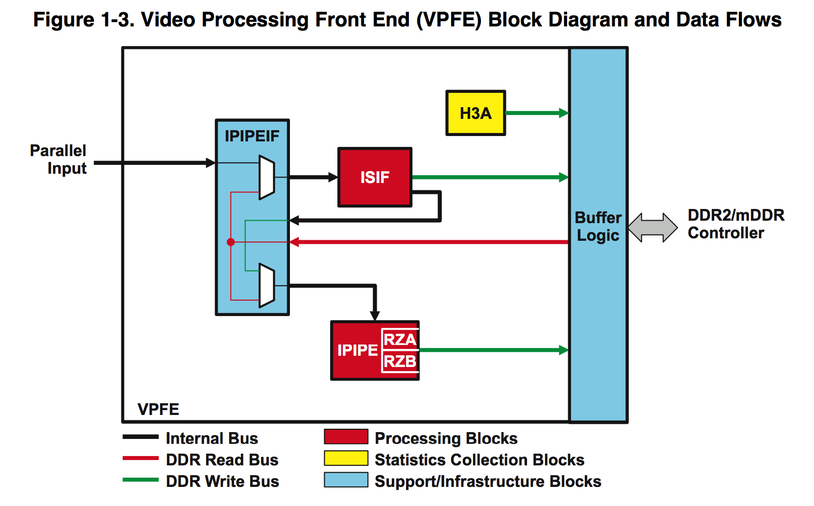
look at it: IPIPEIF (Image Pipe Interface) receives a “raw” raw 12 bit picture inBayer format from the sensor. This block itself does nothing particularly useful, it mainly serves to synchronize the operation of ISIF and IPIPE, and can also subtract a “dark” memory from each new frame, but we do not use it.
Image Sensor Interface (ISIF) can convert Bayer to various formats, multiply, subtract, etc., for more details on the possibilities can be found in the documentation . We use from this block for our algorithms:
1. “Subtractor” of a constant value from all colors, for our two sensors in total darkness, not 0, but a constant is output, for SONY 176, but for Aptina 172. This must be taken into account for proper color balancing especially in the dark.
2. Gain and Offset - to them we do white balance. For each color, you can set your own multiplication factor from 0 to (7 + 511/512), in the standard format for all hardware “multipliers”: OUT = IN * G >> 9, where IN is the input color value, G is “multiplier” from 0 to 4095.
The next Image Pipe (IPIPE) block is used by us for everything else.
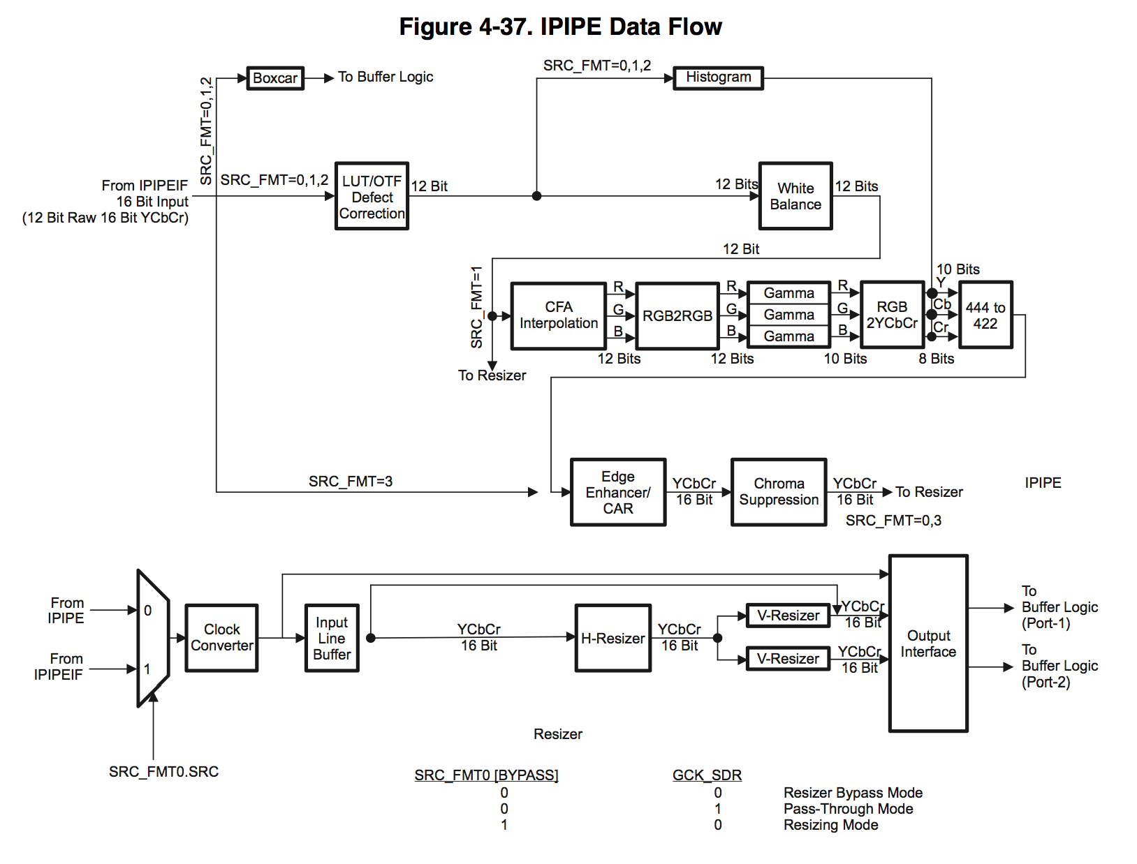
Let's start in order:
1. Defect Correction can process “broken” pixels, though before processing it must know their coordinates, and to set them, it is necessary to calibrate each sensor in the dark, which greatly complicates the production. Not so many defective sensors come across, and if you get caught - it's easier to replace.
2. The next White Balance block consists of 3 multipliers and 3 x subtractors, one for each color, we use it as a global multiplication factor and a threshold subtractor, the same for all colors.
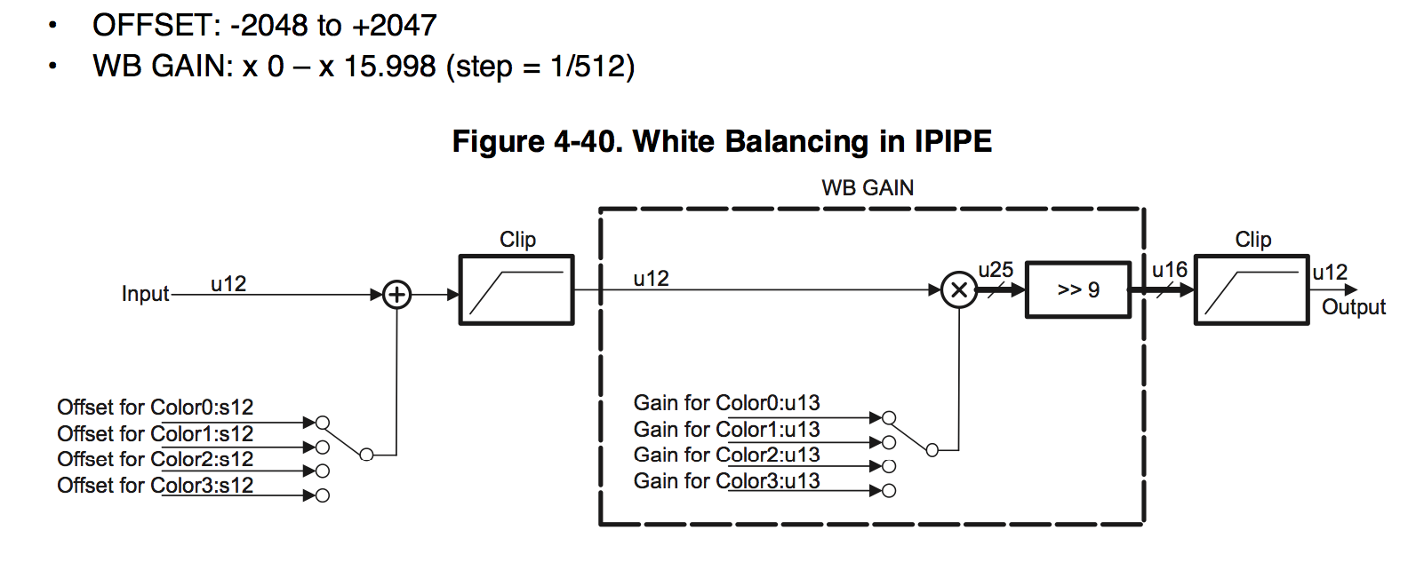
the format is the same as in the ISIF block, only the multiplication range is twice as large.
3. CFA Interpolation Converts From Bayer Format
What interpolation algorithm is used, we have not found.
4. RGB2RGB blending module passes each RGB pixel through a matrix

where gain can vary from -8 to +7.996 in increments of 1/256 = 0.004, and offset from -4096 to 4095.
Moreover, there were two of these blocks, one after the other, and we got them we use both in our algorithms. Each manufacturer gives tables for its sensors. Honestly, I don’t quite understand how it works, and how colors can mix, but the picture really gets better. Soon you will see for yourself.
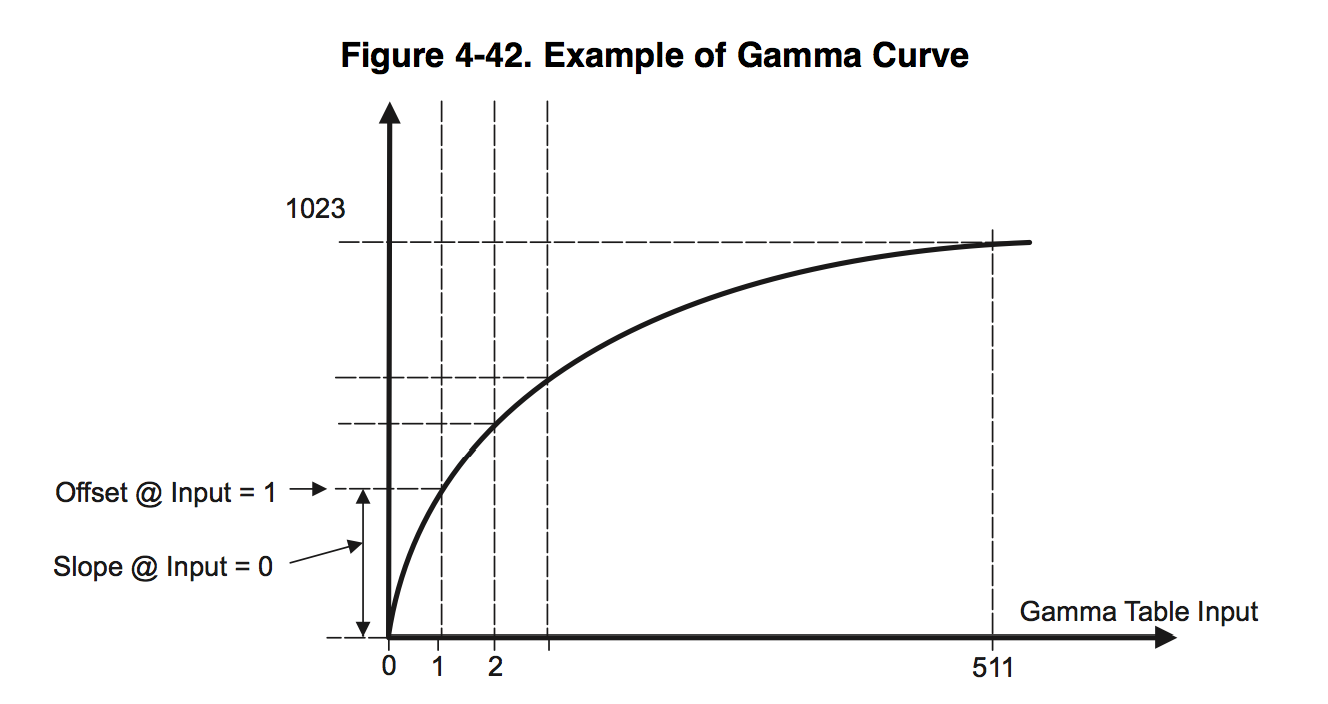
5. The gamma correction block consists of 3 LUTs (look-up-table), one for each color.
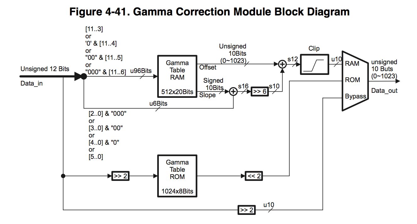
You can select a table size from 512 to 64 values, we use 512. Each table element consists of two 10 bit words Offset and Slope.
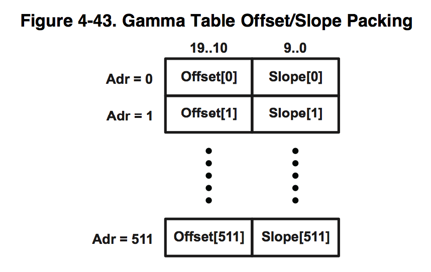
The input receives 12 bit IN data, then it is divided into two parts HIGH = IN >> 3, LOW = IN & 7, the upper 9 bits and the lower 3 bits. The output value is calculated using the following formula OUT = (Offset [HIGH] << 3) + (Slope [HIGH] >> 3) * LOW. That is, the gamma curve is approximated by a piecewise smooth function.
6. The RGB2YCbCr block converts the RGB color space to YCbCr.
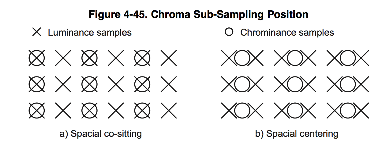
7. 4: 2: 2 Conversion Module halves the color components of Cb and Cr
horizontally.
8. 2D Edge Enhancer, this is a 5x5 two-dimensional filter that improves image contrast - this is a separate topic for the article, here are only examples of its work:
2D EE off:
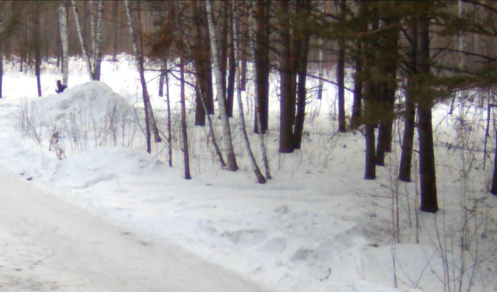
2D EE on:
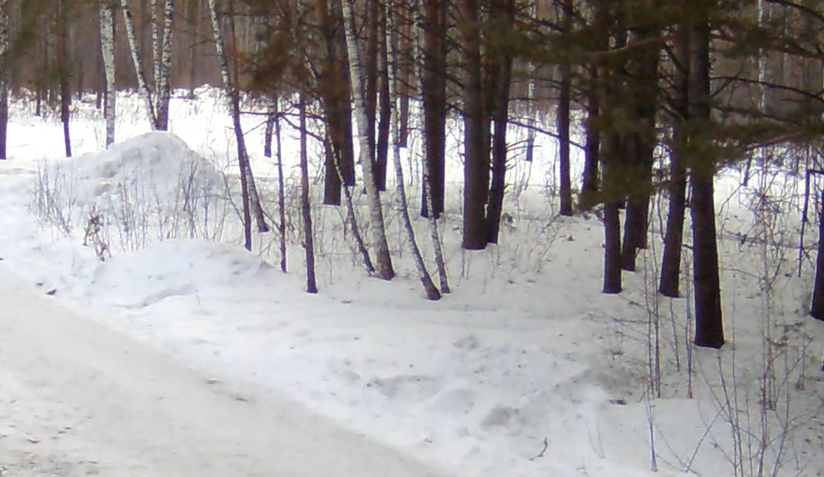
That is a very useful thing.
9. Resizer reduces the image vertically and horizontally for the second and third streams, and also converts the YCbCr 422 to YCbCr 420 for the encoder.
Separate from the entire video processing path is the H3A statistics block. It is needed to implement all the algorithms. Based on the data received from it, exposure, gain and shift are set.
1. Statistics for exposure and color balance are obtained by dividing the picture into cells up to 56 horizontally and 128 vertically. For each cell, you can get the sum of all the pixels for each color, their minimum and maximum values.
2. The autofocus block also splits the picture into cells up to 12 horizontally and 128 vertically. And for each cell gives the maximum focus value.
But they didn’t explain what it was. Studying the software didn’t clarify anything much, it only became known that it was a certain RIF filter, where coefficients and thresholds could be changed, but it didn’t help much, and autofocus was not stable.
So, why did we take it and what did not suit us in existing algorithms? The main problem of the existing algorithm is the incomplete use of the dynamic range.
An example of the algorithm working in cloudy weather:

In the mornings and evenings, as a rule, the white balance floats:
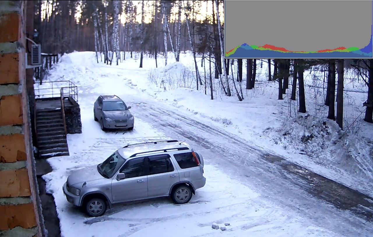
And this example with our algorithm:
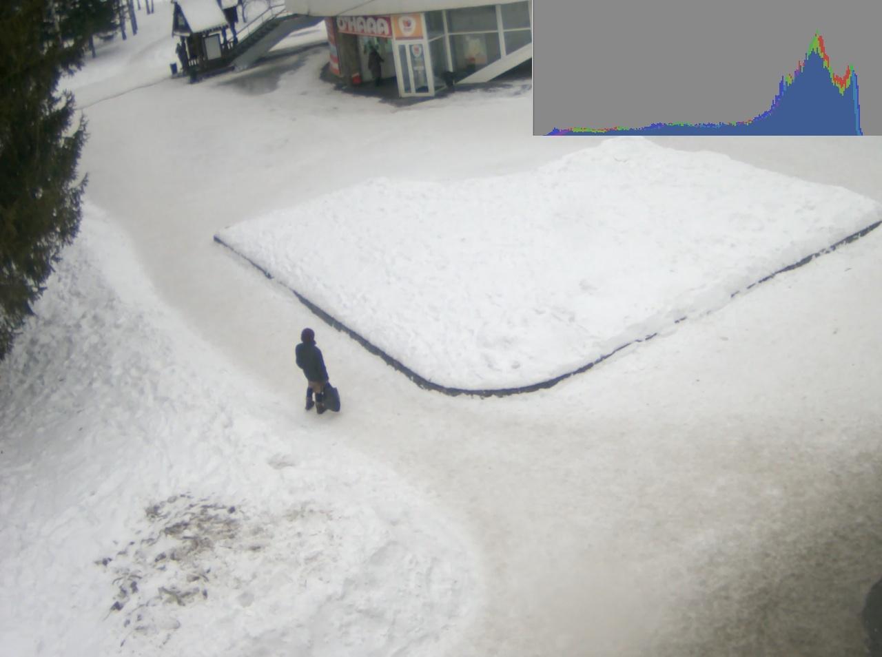
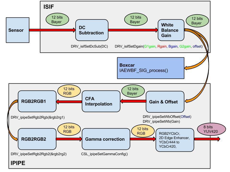
And so that everything worked well with different sensors, we decided not to edit a bunch of other people's software, but to write our own from scratch. Another task of the algorithm should be as easily as possible transferred to other platforms. Fortunately, the DM368 turned out to have a very useful hardware unit, the so-called Boxcar. It’s nothing more than an averager with 8x8 or 16x16 blocks.

That is, at the output of boxcar we get a 16-bit reduced raw image on each axis. If the input resolution is 1920x1080, then for statistics we have 120x68.
We took this block as a source of statistics.
Let's draw a block diagram of our algorithm and move on to the code.
You can watch the live broadcast from our and other people's cameras here .
To be continued…
Let us examine the main blocks of video stream processing from the sensor to the network “broadcaster”, we will dwell in more detail on the algorithms of autoexposure, white balance and autofocus (3A), gamma correction, as well as the extended dynamic range of HDR or WDR, and finally, motion detection and analytics on its basis.
Examples of pictures will be presented for the SONY IMX136 sensor , the algorithm is also tested on Aptina MT9P006 , AR0331 , MT9M034 sensors .
| Before | After |
 |  |
The main players in the processor market for ip video surveillance are 3 companies TI , Ambarella and Hisilicon . All of them have chips of different price ranges, the most popular on the market right now with the ability to encode FHD (1920x1080) video stream up to 30 frames per second DM368 (TI), A5 (Ambarella), Hi3516 (Hisilicon) at a price of $ 10 to $ 20 and more powerful up to 60 frames per second DM385 (TI), A7 (Ambarella), Hi3517 (Hisilicon) at a price of $ 20 to $ 40. The characteristics of these chips are approximately the same.
Since TI is a fairly open company, all the hardware documentation is on the site, it is easiest to work with. To get the software and the whole design, just buy a camera from Approfor $ 1,000 and more. To obtain documentation from HiSilicon, you must sign an NDA, and the cost of support and a reference fee is $ 5,000. The most expensive was Ambarella, to get the documentation and support you need to shell out $ 25,400.
So, back to DM368:
As you can see in the diagram, the processor has everything that is needed for the ip camera and not only for it. Video Processing Subsystem (VPSS) is involved in video processing; in turn, it consists of two Video FE (Front End) and Video BE (Back End) blocks. Video FE is responsible for inputting and processing a video signal, and Video BE for encoding and output to various devices. Hardware support for 3A algorithms is located in the Video FE module.
Let's take a closer
look at it: IPIPEIF (Image Pipe Interface) receives a “raw” raw 12 bit picture inBayer format from the sensor. This block itself does nothing particularly useful, it mainly serves to synchronize the operation of ISIF and IPIPE, and can also subtract a “dark” memory from each new frame, but we do not use it.
Image Sensor Interface (ISIF) can convert Bayer to various formats, multiply, subtract, etc., for more details on the possibilities can be found in the documentation . We use from this block for our algorithms:
1. “Subtractor” of a constant value from all colors, for our two sensors in total darkness, not 0, but a constant is output, for SONY 176, but for Aptina 172. This must be taken into account for proper color balancing especially in the dark.
2. Gain and Offset - to them we do white balance. For each color, you can set your own multiplication factor from 0 to (7 + 511/512), in the standard format for all hardware “multipliers”: OUT = IN * G >> 9, where IN is the input color value, G is “multiplier” from 0 to 4095.
The next Image Pipe (IPIPE) block is used by us for everything else.
Let's start in order:
1. Defect Correction can process “broken” pixels, though before processing it must know their coordinates, and to set them, it is necessary to calibrate each sensor in the dark, which greatly complicates the production. Not so many defective sensors come across, and if you get caught - it's easier to replace.
2. The next White Balance block consists of 3 multipliers and 3 x subtractors, one for each color, we use it as a global multiplication factor and a threshold subtractor, the same for all colors.
the format is the same as in the ISIF block, only the multiplication range is twice as large.
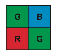
3. CFA Interpolation Converts From Bayer Format
 | in RGB | 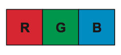 |
What interpolation algorithm is used, we have not found.
4. RGB2RGB blending module passes each RGB pixel through a matrix
where gain can vary from -8 to +7.996 in increments of 1/256 = 0.004, and offset from -4096 to 4095.
Moreover, there were two of these blocks, one after the other, and we got them we use both in our algorithms. Each manufacturer gives tables for its sensors. Honestly, I don’t quite understand how it works, and how colors can mix, but the picture really gets better. Soon you will see for yourself.
5. The gamma correction block consists of 3 LUTs (look-up-table), one for each color.
You can select a table size from 512 to 64 values, we use 512. Each table element consists of two 10 bit words Offset and Slope.
The input receives 12 bit IN data, then it is divided into two parts HIGH = IN >> 3, LOW = IN & 7, the upper 9 bits and the lower 3 bits. The output value is calculated using the following formula OUT = (Offset [HIGH] << 3) + (Slope [HIGH] >> 3) * LOW. That is, the gamma curve is approximated by a piecewise smooth function.
6. The RGB2YCbCr block converts the RGB color space to YCbCr.
7. 4: 2: 2 Conversion Module halves the color components of Cb and Cr
horizontally.
8. 2D Edge Enhancer, this is a 5x5 two-dimensional filter that improves image contrast - this is a separate topic for the article, here are only examples of its work:
2D EE off:
2D EE on:
That is a very useful thing.
9. Resizer reduces the image vertically and horizontally for the second and third streams, and also converts the YCbCr 422 to YCbCr 420 for the encoder.
Separate from the entire video processing path is the H3A statistics block. It is needed to implement all the algorithms. Based on the data received from it, exposure, gain and shift are set.
1. Statistics for exposure and color balance are obtained by dividing the picture into cells up to 56 horizontally and 128 vertically. For each cell, you can get the sum of all the pixels for each color, their minimum and maximum values.
2. The autofocus block also splits the picture into cells up to 12 horizontally and 128 vertically. And for each cell gives the maximum focus value.
But they didn’t explain what it was. Studying the software didn’t clarify anything much, it only became known that it was a certain RIF filter, where coefficients and thresholds could be changed, but it didn’t help much, and autofocus was not stable.
So, why did we take it and what did not suit us in existing algorithms? The main problem of the existing algorithm is the incomplete use of the dynamic range.
An example of the algorithm working in cloudy weather:
In the mornings and evenings, as a rule, the white balance floats:
And this example with our algorithm:
And so that everything worked well with different sensors, we decided not to edit a bunch of other people's software, but to write our own from scratch. Another task of the algorithm should be as easily as possible transferred to other platforms. Fortunately, the DM368 turned out to have a very useful hardware unit, the so-called Boxcar. It’s nothing more than an averager with 8x8 or 16x16 blocks.
That is, at the output of boxcar we get a 16-bit reduced raw image on each axis. If the input resolution is 1920x1080, then for statistics we have 120x68.
We took this block as a source of statistics.
Let's draw a block diagram of our algorithm and move on to the code.
You can watch the live broadcast from our and other people's cameras here .
To be continued…