December 2, 2013 at 15:07
An example of solving a credit scoring problem using the python + pandas + scikit-learn bundle
Introduction
Good afternoon, dear readers.
Recently, wandering around the expanses of the global web, I came across a tournament that was held by the TCS bank earlier this year. After reviewing the tasks, I decided to test my skills in analyzing data on them.
I decided to start the verification with the scoring problem (Task number 3). To solve it, I, as always, used Python with the pandas and scikit-learn analytic modules .
Description of the data and statement of the problem
The Bank requests the credit history of the applicant from the three largest Russian credit bureaus. A selection of Bank customers is provided in the SAMPLE_CUSTOMERS.CSV file . The sample is divided into parts "train" and "test". From the “train” sample, the value of the bad target variable is known - the presence of "default" (the client assumes a delay of 90 days or more during the first year of using the loan). The file SAMPLE_ACCOUNTS.CSV provides data from the responses of credit bureaus to all requests for relevant customers. SAMPLE_CUSTOMERS
data format - information about the possibility of default of a particular person.
Description of SAMPLE_ACCOUNTS dataset format :
Set Description
| Name | Description |
|---|---|
| TCS_CUSTOMER_ID | Customer id |
| BUREAU_CD | Code of the bureau from which the invoice was received |
| BKI_REQUEST_DATE | Date on which the request was made to the bureau |
| Currency | Contract currency (ISO currency letter code) |
| RELATIONSHIP | Type of relationship to contract |
| 1 - Individual | |
| 2 - Additional card / Authorized user | |
| 4 - Joint | |
| 5 - Guarantor | |
| 9 - Legal entity | |
| OPEN_DATE | Contract opening date |
| FINAL_PMT_DATE | Final payment date (planned) |
| Type | Contract Type Code |
| 1 - Car loan | |
| 4 - Leasing | |
| 6 - Mortgage | |
| 7 - Credit Card | |
| 9 - Consumer loan | |
| 10 - Business Development Credit | |
| 11 - Loan for replenishment of working capital | |
| 12 - Loan for the purchase of equipment | |
| 13 - Real estate construction loan | |
| 14 - Credit for the purchase of shares (for example, margin lending) | |
| 99 - Other | |
| PMT_STRING_84M | Discipline (timeliness) of payments. The line is composed of account status codes at the moments when the bank transmits data on the account to the bureau, the first character is the status as of the date PMT_STRING_START, then sequentially in descending order of dates. |
| 0 - New, no rating possible | |
| X - No information | |
| 1 - Payment without delay | |
| A - Delay from 1 to 29 days | |
| 2 - Delay from 30 to 59 days | |
| 3 - Delay from 60 to 89 days | |
| 4 - Delay from 90 to 119 days | |
| 5 - Delay more than 120 days | |
| 7 - Regular consolidated payments | |
| 8 - Repayment of the loan using collateral | |
| 9 - Bad debt / transferred to collection / missed payment | |
| Status | Contract status |
| 00 - Active | |
| 12 - Paid by security | |
| 13 - Account closed | |
| 14 - Transferred to another bank for servicing | |
| 21 - Dispute | |
| 52 - Expired | |
| 61 - Return Issues | |
| OUTSTANDING | Remaining outstanding debt. Amount in rubles at the rate of the Central Bank of the Russian Federation |
| NEXT_PMT | The size of the next payment. Amount in rubles at the rate of the Central Bank of the Russian Federation |
| INF_CONFIRM_DATE | Date of confirmation of account information |
| FACT_CLOSE_DATE | Account Closing Date (Actual) |
| TTL_DELQ_5 | The number of delays up to 5 days |
| TTL_DELQ_5_29 | The number of delays from 5 to 29 days |
| TTL_DELQ_30_59 | The number of delays from 30 to 59 days |
| TTL_DELQ_60_89 | The number of delays from 60 to 89 days |
| TTL_DELQ_30 | The number of delays up to 30 days |
| TTL_DELQ_90_PLUS | The number of delays 90+ days |
| PMT_FREQ | Payment Frequency Code |
| 1 - Weekly | |
| 2 - Once every two weeks | |
| 3 - Monthly | |
| A - Once every 2 months | |
| 4 - Quarterly | |
| B - Once every 4 months | |
| 5 - Once every six months | |
| 6 - Annually | |
| 7 - Other | |
| CREDIT_LIMIT | Credit limit. Amount in rubles at the rate of the Central Bank of the Russian Federation |
| DELQ_BALANCE | Current arrears. Amount in rubles at the rate of the Central Bank of the Russian Federation |
| MAX_DELQ_BALANCE | The maximum amount of arrears. Amount in rubles at the rate of the Central Bank of the Russian Federation |
| CURRENT_DELQ | Current number of days past due |
| PMT_STRING_START | Line Start Date PMT_STRING_84M |
| INTEREST_RATE | Loan interest rate |
| CURR_BALANCE_AMT | The total amount paid, including the principal amount, interest, penalties and fines. Amount in rubles at the rate of the Central Bank of the Russian Federation |
The task is to build a model on the “train” sample that determines the probability of “default” and put down its probabilities for customers from the “test” sample . To evaluate the model, the Area Under ROC Curve characteristic will be used (also indicated in the task conditions).
Data preprocessing
To get started, download the source files and look at them:
from pandas import read_csv, DataFrame
from sklearn.metrics import roc_curve
from sklearn.ensemble import RandomForestClassifier, GradientBoostingClassifier
from sklearn.cross_validation import train_test_split
from sklearn.naive_bayes import GaussianNB
from sklearn.neighbors import KNeighborsClassifier
from sklearn.decomposition import PCA
import ml_metrics, string, re, pylab as pl
SampleCustomers = read_csv("https://static.tcsbank.ru/documents/olymp/SAMPLE_CUSTOMERS.csv", ';')
SampleAccounts = read_csv("https://static.tcsbank.ru/documents/olymp/SAMPLE_ACCOUNTS.csv",";",decimal =',')
print SampleAccounts
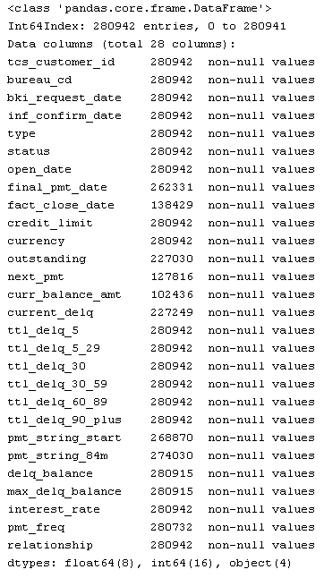
SampleCustomers.head()| tcs_customer_id | bad | sample_type | |
|---|---|---|---|
| 0 | 1 | NaN | test |
| 1 | 2 | 0 | train |
| 2 | 3 | 1 | train |
| 3 | 4 | 0 | train |
| 4 | 5 | 0 | train |
From the conditions of the task, we can assume that the SampleAccounts set contains several records for one borrower, let's check this:
SampleAccounts.tcs_customer_id.drop_duplicates().count(), SampleAccounts.tcs_customer_id.count()Our assumption was correct. Unique borrowers 50,000 of 280,942 records. This is due to the fact that one borrower has several loans and for each of them different information in different bureaus. Therefore, you need to perform conversions on SampleAccounts so that one line corresponds to one borrower.
Now let's get a list of all unique loans for each borrower:
SampleAccounts[['tcs_customer_id','open_date','final_pmt_date','credit_limit','currency']].drop_duplicates()Therefore, when we received the list of loans, we can display some general information for each element of the list. Those. it would be possible to take a bunch of the fields listed above and make it an index, against which we would perform further manipulations, but, unfortunately, one unpleasant moment lies in wait for us. It consists in the fact that the 'final_pmt_date' field in the dataset has empty values. Let's try to get rid of them.
We have in the set the field the actual closing date of the loan, therefore, if it is, and the field 'final_pmt_date' is not filled, then you can write this value into it. For the rest, just write 0.
SampleAccounts.final_pmt_date[SampleAccounts.final_pmt_date.isnull()] = SampleAccounts.fact_close_date[SampleAccounts.final_pmt_date.isnull()].astype(float)
SampleAccounts.final_pmt_date.fillna(0, inplace=True)
Now that we have got rid of empty values, let's get the latest date for contacting any of the bureaus for each of the loans. This is useful to us for determining its attributes, such as contract status, type, etc.
sumtbl = SampleAccounts.pivot_table(['inf_confirm_date'],  ['tcs_customer_id','open_date','final_pmt_date','credit_limit','currency'], aggfunc='max')
sumtbl.head(15)
| inf_confirm_date | |||||
|---|---|---|---|---|---|
| tcs_customer_id | open_date | final_pmt_date | credit_limit | currency | |
| 1 | 39261 | 39629 | 19421 | RUB | 39924 |
| 39505 | 39870 | 30000 | RUB | 39862 | |
| 39644 | 40042 | 11858 | RUB | 40043 | |
| 39876 | 41701 | 300,000 | RUB | 40766 | |
| 39942 | 40308 | 19691 | RUB | 40435 | |
| 40421 | 42247 | 169000 | RUB | 40756 | |
| 40428 | 51386 | 10,000 | RUB | 40758 | |
| 40676 | 41040 | 28967 | RUB | 40764 | |
| 2 | 40472 | 40618 | 7551 | RUB | 40661 |
| 40652 | 40958 | 21186 | RUB | 40661 | |
| 3 | 39647 | 40068 | 22694 | RUB | 40069 |
| 40604 | 0 | 20000 | RUB | 40624 | |
| 4 | 38552 | 40378 | 75,000 | RUB | 40479 |
| 39493 | 39797 | 5000 | RUB | 39823 | |
| 39759 | 40123 | 6023 | RUB | 40125 |
Now add the dates we received to the main set:
SampleAccounts = SampleAccounts.merge(sumtbl, 'left',
                                     left_on=['tcs_customer_id','open_date','final_pmt_date','credit_limit','currency'],
                                     right_index=True,
                                     suffixes=('', '_max'))
So, further we will break the columns in which the parameters are strictly defined, so that each value from these fields has a separate column. By condition, the columns with the given values will be:
- pmt_string_84m
- pmt_freq
- type
- status
- relationship
- bureau_cd
The code to convert them is shown below:
# преобразуем pmt_string_84m
vals = list(xrange(10)) + ['A','X']
PMTstr = DataFrame([{'pmt_string_84m_%s' % (str(j)): str(i).count(str(j)) for j in vals} for i in SampleAccounts.pmt_string_84m])
SampleAccounts = SampleAccounts.join(PMTstr).drop(['pmt_string_84m'], axis=1)
# преобразуем pmt_freq
SampleAccounts.pmt_freq.fillna(7, inplace=True)
SampleAccounts.pmt_freq[SampleAccounts.pmt_freq == 0] = 7
vals = list(range(1,8)) + ['A','B']
PMTstr = DataFrame([{'pmt_freq_%s' % (str(j)): str(i).count(str(j)) for j in vals} for i in SampleAccounts.pmt_freq])
SampleAccounts = SampleAccounts.join(PMTstr).drop(['pmt_freq'], axis=1)
# преобразуем type
vals = [1,4,6,7,9,10,11,12,13,14,99]
PMTstr = DataFrame([{'type_%s' % (str(j)): str(i).count(str(j)) for j in vals} for i in SampleAccounts.type])
SampleAccounts = SampleAccounts.join(PMTstr).drop(['type'], axis=1)
# преобразуем status
vals = [0,12, 13, 14, 21, 52,61]
PMTstr = DataFrame([{'status_%s' % (str(j)): str(i).count(str(j)) for j in vals} for i in SampleAccounts.status])
SampleAccounts = SampleAccounts.join(PMTstr).drop(['status'], axis=1)
# преобразуем relationship
vals = [1,2,4,5,9]
PMTstr = DataFrame([{'relationship_%s' % (str(j)): str(i).count(str(j)) for j in vals} for i in SampleAccounts.relationship])
SampleAccounts = SampleAccounts.join(PMTstr).drop(['relationship'], axis=1)
# преобразуем bureau_cd
vals = [1,2,3]
PMTstr = DataFrame([{'bureau_cd_%s' % (str(j)): str(i).count(str(j)) for j in vals} for i in SampleAccounts.bureau_cd])
SampleAccounts = SampleAccounts.join(PMTstr).drop(['bureau_cd'], axis=1)
The next step is to convert the field 'fact_close_date', which contains the date of the last actual payment, so that it contains only 2 values:
- 0 - there was no last payment
- 1 - the last payment was
I made this replacement because initially the field was half full.
SampleAccounts.fact_close_date[SampleAccounts.fact_close_date.notnull()] = 1
SampleAccounts.fact_close_date.fillna(0, inplace=True)
Now we need to get the latest data on all loans from our data set. The "inf_confirm_date_max" field obtained above will help us in this . We added the deadline for updating credit information in all bureaus to it:
PreFinalDS = SampleAccounts[SampleAccounts.inf_confirm_date == SampleAccounts.inf_confirm_date_max].drop_duplicates()After the above actions, our sample was significantly reduced, but now we need to summarize all the information on the loan and the borrower obtained earlier. To do this, we will group our data set:
PreFinalDS = PreFinalDS.groupby(['tcs_customer_id','open_date','final_pmt_date','credit_limit','currency']).max().reset_index()Our data is almost ready to start the analysis. It remains to perform a few more actions:
- Remove unnecessary columns
- Bring all credit limits in rubles
- Calculate how many loans each borrower according to information from the bureau
Let's start by clearing the table of unnecessary columns:
PreFinalDS = PreFinalDS.drop(['bki_request_date',
                              'inf_confirm_date',
                              'pmt_string_start',
                              'interest_rate',
                              'open_date',
                              'final_pmt_date',
                              'inf_confirm_date_max'], axis=1)
Next, we transfer all credit limits to rubles. For simplicity, I took the current exchange rates. Although it would probably be more correct to take a course at the time of opening the account. Another nuance is that for analysis we need to remove the “Сurrency” text field , therefore, after converting currencies into rubles, we will manipulate this field with the fields above:
curs = DataFrame([33.13,44.99,36.49,1], index=['USD','EUR','GHF','RUB'], columns=['crs'])
PreFinalDS = PreFinalDS.merge(curs, 'left', left_on='currency', right_index=True)
PreFinalDS.credit_limit = PreFinalDS.credit_limit * PreFinalDS.crs
#выделяем значения в отдельные столбцы
vals = ['RUB','USD','EUR','CHF']
PMTstr = DataFrame([{'currency_%s' % (str(j)): str(i).count(str(j)) for j in vals} for i in PreFinalDS.currency])
PreFinalDS = PreFinalDS.join(PMTstr).drop(['currency','crs'], axis=1)
So, before the final grouping, we will add a field filled with units to our set. Those. when we do the last grouping, the amount on it will give the number of loans from the borrower:
PreFinalDS['count_credit'] = 1Now that we have all the data in the data set quantitative, you can fill in the gaps in the data 0 and perform the final grouping by customer:
PreFinalDS.fillna(0, inplace=True)
FinalDF = PreFinalDS.groupby('tcs_customer_id').sum()
FinalDF
Preliminary analysis
Well, the primary data processing is completed and you can begin to analyze them. To begin, we will divide our data into training and test samples. The column “sample_type” from SampleCustomers will help us with this , just such a separation has been made.
In order to break our processed DataFrame, just combine it with SampleCustomers to play with filters:
SampleCustomers.set_index('tcs_customer_id', inplace=True)
UnionDF = FinalDF.join(SampleCustomers)
trainDF = UnionDF[UnionDF.sample_type == 'train'].drop(['sample_type'], axis=1)
testDF = UnionDF[UnionDF.sample_type == 'test'].drop(['sample_type'], axis=1)
Next, let's see how the signs correlate with each other, for this we construct a matrix with the correlation coefficients of the signs. With pandas, this can be done with one command:
CorrKoef = trainDF.corr()After the action above, CorrKoef will contain a 61x61 size matrix.
Rows and columns of it will be the corresponding field names, and at their intersection - the value of the correlation coefficient. For instance:
| fact_close_date | |
|---|---|
| status_13 | 0.997362 |
A case is possible when there is no correlation coefficient. This means that these fields are most likely filled with only one identical value and can be omitted during analysis. Check:
FieldDrop = [i for i in CorrKoef if CorrKoef[i].isnull().drop_duplicates().values[0]]
At the output, we got a list of fields that can be deleted:
- pmt_string_84m_6
- pmt_string_84m_8
- pmt_freq_5
- pmt_freq_A
- pmt_freq_B
- status_12
The next step is to find the fields that correlate with each other (for which the correlation coefficient is more than 90%) using our matrix:
CorField = []
for i in CorrKoef:
    for j in CorrKoef.index[CorrKoef[i] > 0.9]:
        if i <> j and j not in CorField and i not in CorField:
            CorField.append(j)
            print "%s-->%s: r^2=%f" % (i,j, CorrKoef[i][CorrKoef.index==j].values[0])
На выходе получим следующие:
fact_close_date-->status_13: r^2=0.997362
ttl_delq_5_29-->ttl_delq_30: r^2=0.954740
ttl_delq_5_29-->pmt_string_84m_A: r^2=0.925870
ttl_delq_30_59-->pmt_string_84m_2: r^2=0.903337
ttl_delq_90_plus-->pmt_string_84m_5: r^2=0.978239
delq_balance-->max_delq_balance: r^2=0.986967
pmt_freq_3-->relationship_1: r^2=0.909820
pmt_freq_3-->currency_RUB: r^2=0.910620
pmt_freq_3-->count_credit: r^2=0.911109
Итак, исходя из связей которые мы получили на предыдущем шаге, мы можем добавить в список удаления следующие поля:
FieldDrop =FieldDrop + ['fact_close_date','ttl_delq_30',
                        'pmt_string_84m_5',
                        'pmt_string_84m_A',
                        'pmt_string_84m_A',
                        'max_delq_balance',
                        'relationship_1',
                        'currency_RUB',
                        'count_credit']
newtr = trainDF.drop(FieldDrop, axis=1)
Построение и выбор модели
Well, what is the primary data processed and now we can proceed to the construction of the model.
Separate the class attribute from the training set:
target = newtr.bad.values
train = newtr.drop('bad', axis=1).values
Now let's reduce the dimension of our sample in order to take only significant parameters. To do this, we use the principal component method and its implementation of PCA () in the sklearn module . In the parameter we pass the number of components that we want to save (I chose 20, because with them the results of the models practically did not differ from the results according to the initial data)
coder = PCA(n_components=20)
train = coder.fit_transform(train)
The time has come to define classification models. Let's take a few different algorithms and compare the results of their work using the characteristics of Area Under ROC Curve ( auc ). For modeling, the following algorithms will be considered:
models = []
models.append(RandomForestClassifier(n_estimators=165, max_depth=4, criterion='entropy'))
models.append(GradientBoostingClassifier(max_depth =4))
models.append(KNeighborsClassifier(n_neighbors=20))
models.append(GaussianNB())
So the models are selected. Let's split our training sample into 2 subsamples: test and training. This action is necessary so that we can calculate the auc characteristic for our models. The splitting can be done with the train_test_split () function from the sklearn module :
TRNtrain, TRNtest, TARtrain, TARtest = train_test_split(train, target, test_size=0.3, random_state=0)It remains to train our models and evaluate the result.
There are 2 ways to calculate auc characteristics :
- By standard means of the sklearn module using the roc_auc_score or auc function
- Using the third-party ml_metrics package and the auc () function
I will use the second method, because The first was shown in a previous article. The ml_metrics package is a very useful addition to sklearn, as it contains some metrics that are not in sklearn.
So, we will build ROC curves and calculate their areas:
plt.figure(figsize=(10, 10))
for model in models:
    model.fit(TRNtrain, TARtrain)
    pred_scr = model.predict_proba(TRNtest)[:, 1]
    fpr, tpr, thresholds = roc_curve(TARtest, pred_scr)
    roc_auc = ml_metrics.auc(TARtest, pred_scr)
    md = str(model)
    md = md[:md.find('(')]
    pl.plot(fpr, tpr, label='ROC fold %s (auc = %0.2f)' % (md, roc_auc))
pl.plot([0, 1], [0, 1], '--', color=(0.6, 0.6, 0.6))
pl.xlim([0, 1])
pl.ylim([0, 1])
pl.xlabel('False Positive Rate')
pl.ylabel('True Positive Rate')
pl.title('Receiver operating characteristic example')
pl.legend(loc="lower right")
pl.show()
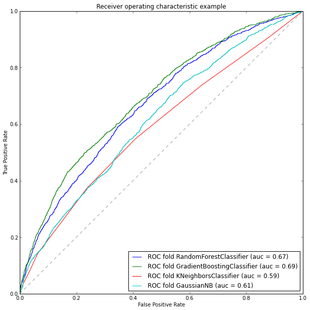
So, according to the results of the analysis of our models, we can say that gradient boosting showed its best, its accuracy is about 69%. Accordingly, for training a test sample, we will choose it. Let's fill in the information in the test sample, pre-processing it to the desired format:
#приводим тестовую выборку к нужному формату
FieldDrop.append('bad')
test = testDF.drop(FieldDrop, axis=1).values
test = coder.fit_transform(test)
#обучаем модель
model = models[1]
model.fit(train, target)
#записываем результат
testDF.bad = model.predict(test)
Conclusion
In conclusion, I would like to note that the obtained model accuracy of 69% is not good enough, but I could not achieve more accuracy. I would like to note the fact that when building the model in full dimension, i.e. excluding correlated columns and dimensionality reduction, it also gave 69% accuracy (this can be easily checked using the trainDF kit for model training)
In this article, I tried to show all the main stages of data analysis from primary processing of raw data to building a classifier model. In addition, I would like to note that the support vector method was not included in the analyzed models, this is due to the fact that after normalizing the data, the accuracy of the model dropped to 51% and the best result that I managed to get with it was around 60%, with significant time cost.
I would also like to note that, unfortunately, the test sample failed to verify the result, because did not meet the dates of the tournament.