Segmentation of satellite images on the example of tree recognition

Automatic recognition of satellite or aerial images is the most promising way to obtain information about the location of various objects on the ground. The refusal of manual segmentation of images is especially relevant when it comes to processing large areas of the earth's surface in a short time.

Recently, I had the opportunity to apply theoretical skills and try myself in the field of machine learning on a real project of image segmentation. The goal of the project is the recognition of forest plantations, namely tree crowns on high resolution satellite images. Under the cut, I will share the experience and results.

When it comes to image processing, then segmentation can be given the following definition - it is the finding on the image of characteristic areas that are equally described in a given feature space.

There are luminance, contour, texture and semantic segmentation.

Semantic (or semantic) image segmentation consists in selecting areas on the image, each of which corresponds to a specific attribute. In general, semantic segmentation tasks are difficult to algorithmize, therefore, for the segmentation of images, convolutional neural networks are now widely used, which show good results.

Formulation of the problem

The problem of binary segmentation is being solved - color images (high resolution satellite imagery) are fed to the input of the neural network, in which areas of pixels belonging to the same class - trees are selected.

Initial data

In my possession there was a set of tiles of satellite images of a rectangular area in which the polygon fits. Inside it and need to look for trees. Polygon or multipolygon represented as a GeoJSON file. In my case, the tiles were in png format of 256 by 256 pixels in true color. (alas, no ik) Numbering of tiles in the form of /zoom/x/y.png.

It is guaranteed that all the tiles in the set are obtained from satellite images taken at about the same time of the year (late spring - early fall depending on the climate of a particular region) and days at a similar angle to the surface, where the presence of slight scattered clouds was allowed.

Data preparation

Since the area of ​​the desired polygon may be less than this rectangular area, the first thing to do is to exclude those tiles that go beyond the boundaries of the polygon. For this, a simple script was written that selects the necessary tiles from the GeoJSON file using the polygon. It works as follows. To begin with, the coordinates of all the vertices of the polygon are converted to tile numbers and added to an array. There is also an offset relative to the origin. For visual control, an image is generated, where one pixel is equal to one tile. The polygon on the image is already filled with the offset using the PIL. After that, the image is transferred to the array, from where the necessary tiles are selected, which fall inside the polygon.

from PIL import Image, ImageDraw
# . . .# Ширина и высота находится из разности номеров правого нижнего и левого верхнего тайлов.
img = Image.new("L", (x, y), 0)
draw = ImageDraw.Draw(img)
# Один пиксель равен тайлу. Пусть нужные тайлы будут белыми. points — вершины полигона.
draw.polygon(points, fill=255)
img.show()
mask = numpy.array(img)
# . . .

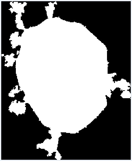
Visual result of converting a polygon into a set of tiles

Network model

To solve the problems of image segmentation, there are a number of models of convolutional neural networks. I decided to use U-Netwhich has proven itself in the problems of binary image segmentation. The U-Net architecture consists of the so-called contracting and an expansive path, which are connected by forwarding at appropriate stages, and first reduce the resolution of the image, and then increase it by first merging it with the image data and passing it through other layers convolutions. Thus, the network serves as a kind of filter. The compressing and unclamping blocks are presented as a set of blocks of a certain dimension. And each block consists of basic operations: convolution, ReLu and max pooling. There are implementations of the U-Net model on Keras, Tensorflow, Caffe and PyTorch. I used Keras.

Creating a training set

Images are required for learning this Unet model. The first thing in my head was the idea to take the data of OpenStreetMap and generate masks for training based on them. But as it turned out in my case, the accuracy of the polygons I need leaves much to be desired. I also needed the presence of single trees, which are not always mapped. Therefore, such an undertaking had to be abandoned. But it should be said, for other objects, such as roads or buildings, this approach can be effective .



Since the idea of ​​automatically generating a training sample based on OSM data had to be abandoned, I decided to manually mark out a small area of ​​terrain. For this, I used the JOSM editor, where as a substrate I used the available images of the terrain, which I placed on a local server. Then another problem surfaced - I could not find an opportunity to turn on the display of the grid of tiles by regular JOSM tools. Therefore, with a couple of simple lines in .htaccess on the same server from another directory, I started issuing an empty pixel-frame tile to any grid-type / z / x / y.png request and added such an improvised layer to JOSM. Such is the bike.



At first I marked out about 30 tiles. With a graphics tablet and “fast drawing mode” in JOSM, it didn't take long. I understood that this amount is not enough for full-fledged training, but I decided to start with this. Moreover, training on such a large amount of data will pass fairly quickly.

Training and the first result

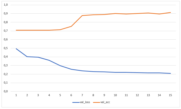
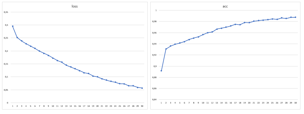
The network has been trained for 15 epochs without prior augmentation of data. The graph shows the values ​​of losses and accuracy on the test sample:



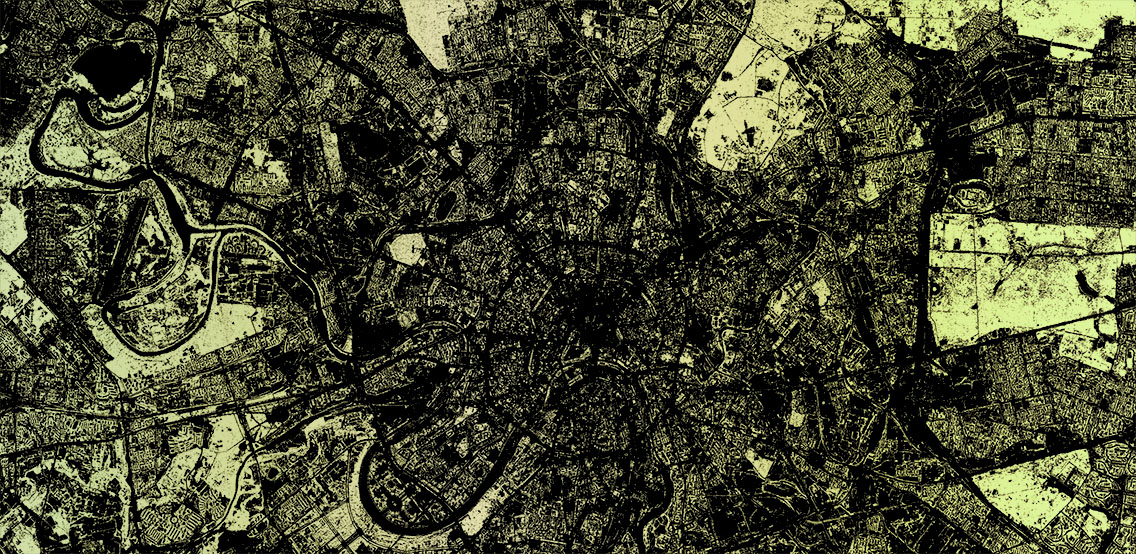
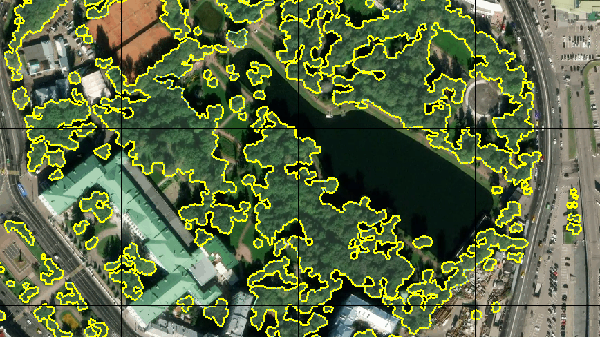
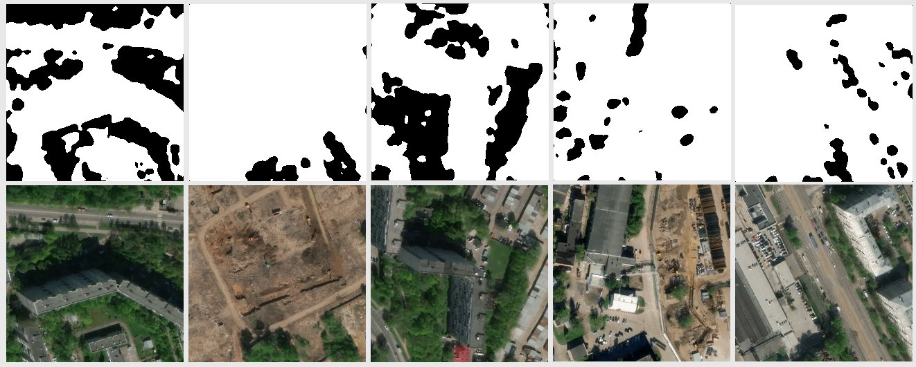
The result of image recognition, which was not in either the training or the test sample, turned out to be quite sane:



After a more thorough study of the results, some problems emerged. A lot of blunders were in the shadow areas of the pictures - the network either found the trees in the shadow where they were not, or exactly the opposite. This was expected, since there were few such examples in the training sample. But I did not expect that some pieces of the water surface and dark metal-roofed roofs (presumably) will be recognized as trees, I did not expect. There were also inaccuracies with lawns. It was decided to improve the sample by adding more images with controversial areas to it, so the learning sample was almost doubled.

Data augmentation

Then I decided to increase the amount of data by turning the images at an arbitrary angle. First of all, I tried the standard keras.preprocessing.image.ImageDataGenerator module. When rotated while maintaining the scale at the edges of the images, empty areas remain, the fill of which is set by the fill_mode parameter . You can simply fill these areas with color, indicating it in cval , but I wanted a full-fledged turn, hoping that the sample would be more complete, and implemented the generator myself. This allowed to increase the size of more than ten times.


fill_mode = nearest

My data generator sticks four adjacent tiles into one source, 512x512 px in size. The angle of rotation is chosen randomly, taking into account it, the admissible intervals for x and y for the center of the resulting tile are calculated, being in which it will not go beyond the limits of the original tile. The coordinates of the center are chosen randomly, taking into account the allowable intervals. Of course, all these transformations are applied to a pair of tile mask. All this is repeated for different groups of neighboring tiles. With one group, you can get more than a dozen tiles with different parts of the area turned at different angles.

# Поворот изображения и вырезка нужной области# image — исходное изображение, center (x, y) — центр необходимой области, a — угол в градусах, width и height — размеры результирующего изображения.
shape = image.shape[:2]
matrix = cv2.getRotationMatrix2D( center=center, angle=a, scale=1 )
image = cv2.warpAffine( src=image, M=matrix, dsize=shape )
x = int( center[0] - width/2  )
y = int( center[1] - height/2 )
image = image[ y:y+height, x:x+width ] # результат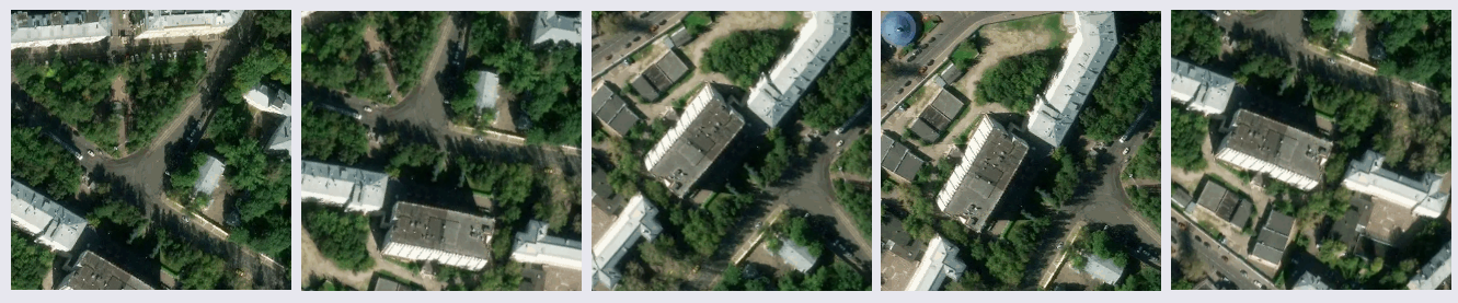

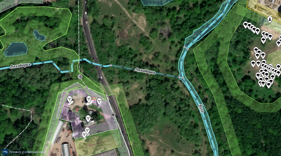
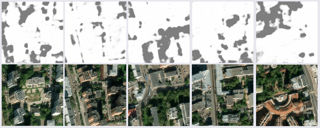
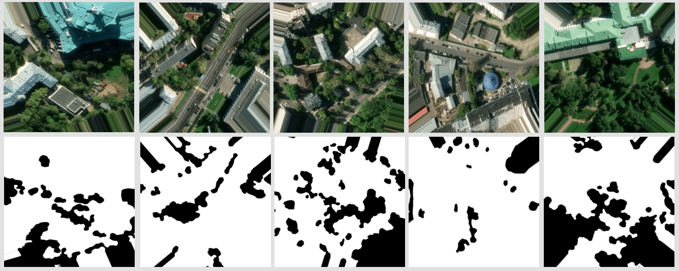
An example of the result of the generator

Learning with more data

As a result, the size of the training sample was 1881 images, I also increased the number of epochs to 30:



After training the model, the problem with erroneous segmentation of roofs and water was no longer detected on the new data volume. It was not possible to get rid of errors in the shadows at all, but their eyes became less, as well as errors with lawns. It should be noted that, in general, the overwhelming majority of errors consist in the fact that the network sees the trees where they are not, and not vice versa. The achieved accuracy can be improved by using satellite images with a large number of channels and modification of the network architecture for a specific task.



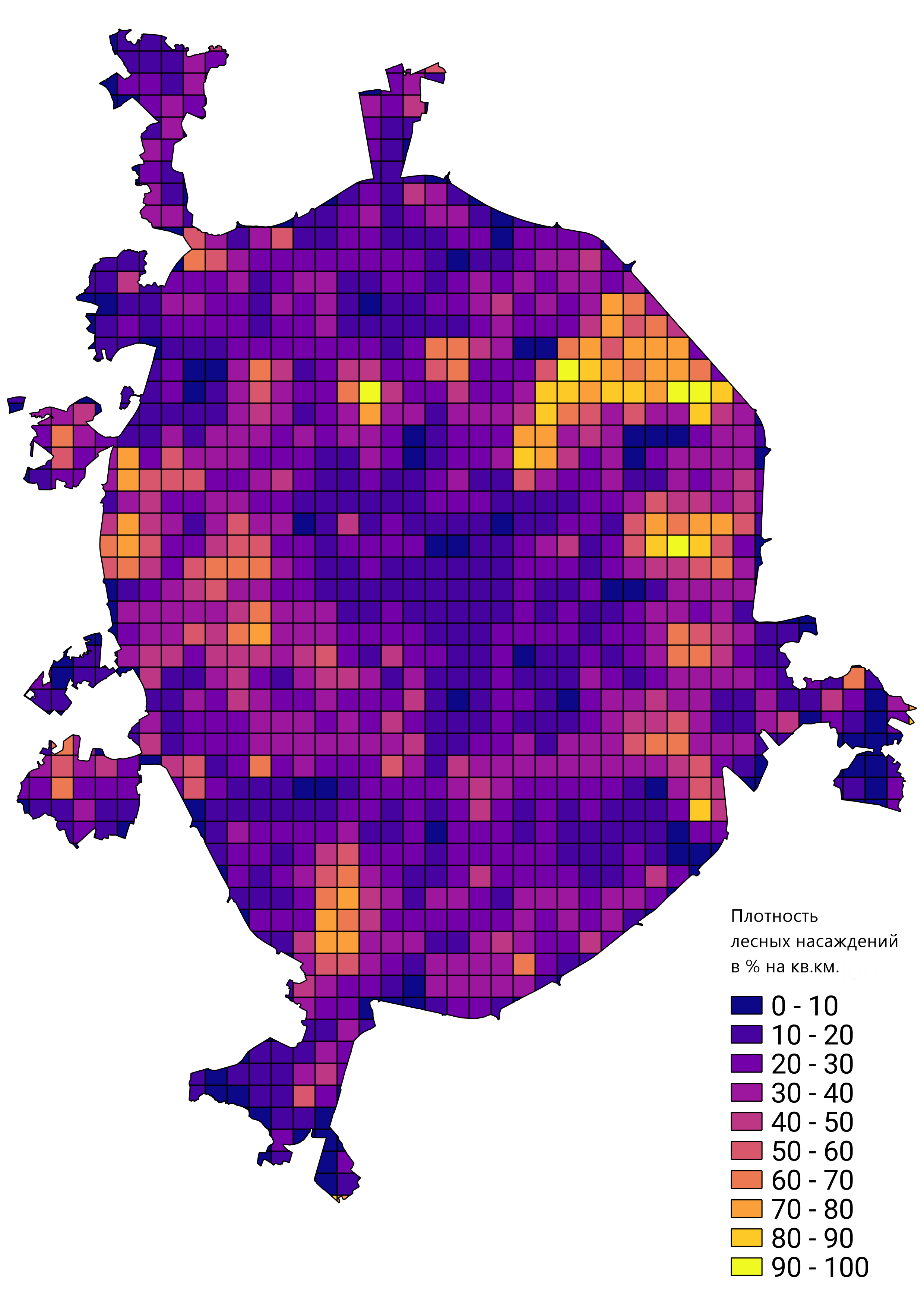
In general, I was satisfied with the result of the work done, and the trained network prototype was used to solve real-world problems. For example, counting the density of forest plantations in Moscow: