1000-dimensional cube: is it possible to create a computational model of human memory today?
- Transfer
This morning, on the way to the Berkeley campus, I ran my fingers through the leaves of a fragrant bush, and then inhaled the familiar smell. I do it every day, and every day the first word that pops up in my head and waves a hand in greeting is sage . But I know that this plant is not sage, but rosemary, so I order the sage to calm down. But too late. After rosemary and sage, I cannot prevent parsley (parsley) and thyme (thyme) from appearing on the stage , after which the first notes of melody and face appear on the album cover in my head, and now I was back in the mid-1960s, wearing a shirt with cucumbers. Meanwhile, rosemarycalls Rose Rose Woods and a 13-minute space (although now , after consulting with the collective memory, I know that this should be Rose Mary Woods and a space of 18 and a half minutes ). From Watergate, I jump to stories on the main page. Then I notice another plant in a well-kept garden with fluffy gray-green leaves. This, too, is not sage, but chisté (lamb's ear). However, sage finally gets its moment of glory. From grass, I am transferred to the Sage math software , and then to the 1950s air defense system called SAGE , Semi-Automatic Ground Environment, which was managed by the largest computer ever built.
In psychology and literature, such mental wanderings are called the stream of consciousness (the author of this metaphor is William James). But I would choose another metaphor. My consciousness, as far as I feel, does not flow smoothly from one topic to another, but rather flits along the landscape of thoughts, more like a butterfly than a river, sometimes nailed to one flower, and then to another, sometimes carried away in gusts by a branch sometimes visiting same place over and over again.
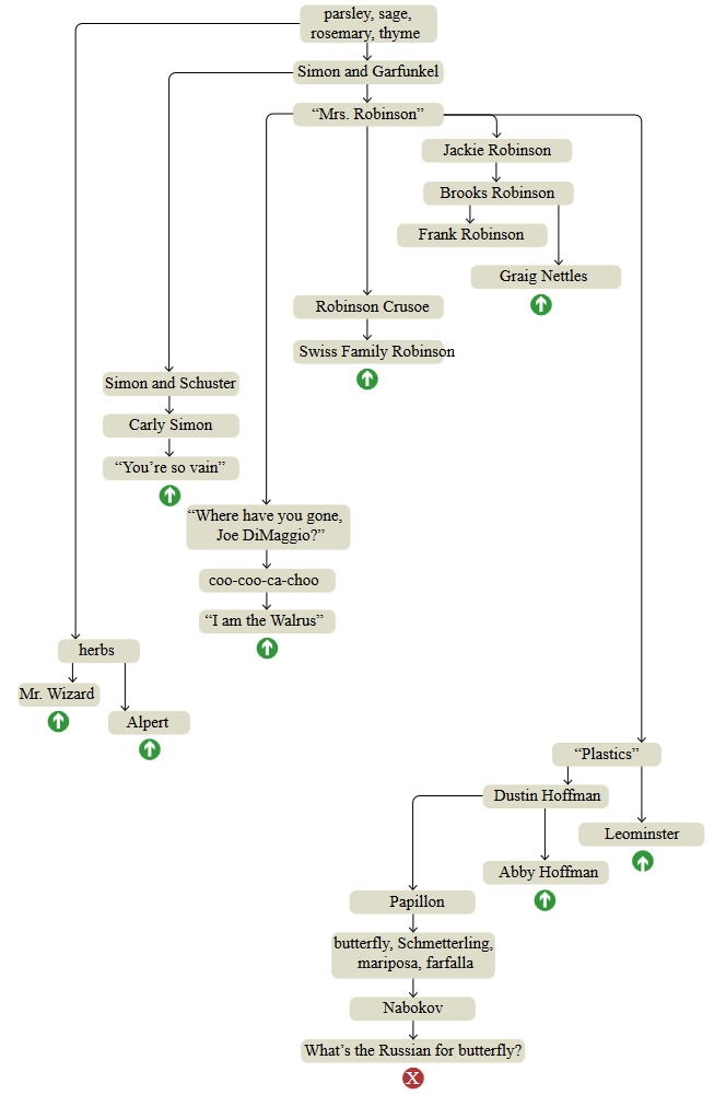
To explore the architecture of my own memory, I tried to conduct a more leisurely experiment with free associations. I started with the same floral recipe — parsley, sage, rosemary and thyme — but for this exercise I did not walk in the Berkeley Hills gardens; I sat at the table and took notes. The diagram below represents the best attempt at reconstructing the full course of my thinking.
parsley, sage, rosemary, thyme - four herbs, as well as a line from the song Simon and Garfunkel.
Simon and Garfunkel - Paul Simon and Art Garfunkel, duet of folk-rock singers of the 1960s and 70s.
Mrs. Robinson is a Simon and Garfunkel song, as well as a character from Mike Nichols' movie The Graduate.
“Where have you gone, Joe DiMaggio?” Is the question asked in “Mrs. Robinson.
Simon and Schuster is a publishing house founded in 1924 by Richard Simon and Max Schuster (originally for publishing crossword puzzles).
Jackie Robinson is a legendary Brooklyn Dodgers player.
Robinson Crusoe - Daniel Defoe's novel about a shipwrecked (1719).
The Swiss Robinson family - Johann David Weiss' novel about the shipwrecked (1812).
herbs (herbs) - fragrant plants
Mr. Wizard is the Saturday science show of the 1950s for children, hosted by Don Herbert.
Alpert - trumpeter Coat of Arms Alpert.
Plastics is a career development board proposed in The Graduate.
coo-coo-ca-choo - a line from "Mrs. Robinson.
Frank Robinson - Baltimore Orioles outfielder in the 1970s.
Graig Nettles is the third baseman of the New York Yankees in the 1970s.
Dustin Hoffman is an actor who has played The Graduate.
Abby Hoffman - “Yipee!”
Leominster is a city in Massachusetts that became the cradle of plastics production in the United States.
Brooks Robinson is the third baseman of the Baltimore Orioles in the 1970s.
Papillon (“The Moth”) - a 1973 film in which Dustin Hoffman played a minor role; "Papillon" in French "butterfly".
Nabokov - Vladimir Nabokov, a born in Russia writer and butterfly studying entomologist.
butterfly, Schmetterling, mariposa, farfalla - “butterfly” in English, German, Spanish and Italian; it seems that all of them (and the French word too) are of independent origin.
How in Russian is called a butterfly - I do not know. Or did not know when this question arose.
“I am the Walrus” is a 1967 Beatles song that also has the phrase “coo-coo-ca-choo”.
Carly Simon is a singer. No connection with Paul Simon, but is the daughter of Richard Simon.
"You're so vain" - Carly Simon's song.
Top-down graphs are themes in the order in which they surfaced in the brain, but connections between nodes do not create a single linear sequence. The structure resembles a tree with short chains of successive associations, ending with a sharp return to an earlier knot, as if I was dragged back by a stretched rubber band. These interrupts are marked on the chart with green arrows; The red cross below is the place where I decided to complete the experiment.
I apologize to those born after 1990, many of the topics mentioned may seem obsolete or mysterious to you. Explanations are presented under the graph, but I do not think that they will make the associations more understandable. After all, memories are personal, they live inside the head. If you want to collect a collection of ideas that fit your own experience, all you have to do is create your own free association schedule. I highly recommend doing this: you may find that you did not know that you know some things.
The purpose of my daily walk down the hill in Berkeley is the Simons Institute and the course of the theory of computing, in which I participate in a brain-computing and computing program lasting one semester. Such an environment causes thoughts of thoughts. I began to think: how can one build a computational model of the free association process? Among the various tasks proposed for solving artificial intelligence, this one looks pretty simple. There is no need for deep rationalization; all that we need to simulate is just dreams and soaring in the clouds - this is what the brain does when it is not loaded. It seems that such a problem is easy to solve, isn't it?
The first idea that comes to mind (at least in myhead), with respect to the architecture of such a computational model, is a random movement along a mathematical graph or network. Network nodes are elements that are stored in memory — ideas, facts, events — and communications are different types of associations between them. For example, a butterfly node can be associated with a moth, a caterpillar, a monarch, and a mother-of-pearl, as well as transitions mentioned in my schedule, and possibly have less obvious connections, for example, “Australian crawl "," Shrimp "," Mohammed Ali "," pellagrara "," choke " and " stage fright ". The host data structure will contain a list of pointers to all of these associated nodes. Pointers can be numbered from 1 to n; the program will generate a pseudo-random number in this interval and go to the corresponding node in which the whole procedure will start anew.
This algorithm reflects some of the basic characteristics of free associations, but does not take into account many of them. The model assumes that all target nodes are equally likely, which looks implausible. To account for the difference of probabilities, we can define each edge. weight and then make the probabilities proportional to the weights.
Even more complicated is the fact that weights depend on the context - on the recent history of human mental activity. If I did not have a combination of Mrs. Robinson and Jackie Robinson, would I have thought about Joe Di Maggio? And now, as I write this, Joltin 'Joe (DiMaggio's nickname) brings to mind Marilyn Monroe, and then Arthur Miller, and again I cannot stop the train of thought. To reproduce this effect in a computer model, a certain mechanism of dynamic regulation of probabilities of entire categories of nodes will be required, depending on which other nodes have been visited recently.
You should also consider the effects of a new kind of novelty. The model should find a place rubber band, constantly pulling me back to Simon and Garfunkel and Mrs. Robinson. Probably, each recently visited node should be added to the list of target options, even if it is not related to the current node. On the other hand, addiction is also a possibility: too often the recalled thoughts become boring, therefore they must be suppressed in the model.
Another final test: some memories are not isolated facts or ideas, but parts of a story. They have a narrative structure with events unfolding in chronological order. For nodes of such episodic recollections, an edge is required next , and possibly also previous. Such a chain of edges unites all our life, including everything that you remember.
Can such a computational model reproduce my mental wanderings? Data collection for such a model will be quite a long process, and it is not surprising, because it took me a lifetime to fill my skull with an interweaving of herbs, Coats of arms, Simons, Robinsons and Hoffmans. Much more than the amount of data, I care about the laboriousness of the graph traversal algorithm. It is very easy to say: “choose a node according to a set of weighted probabilities”, but when I look at the dirty details of the implementation of this action, I can hardly imagine that something like this happens in the brain.
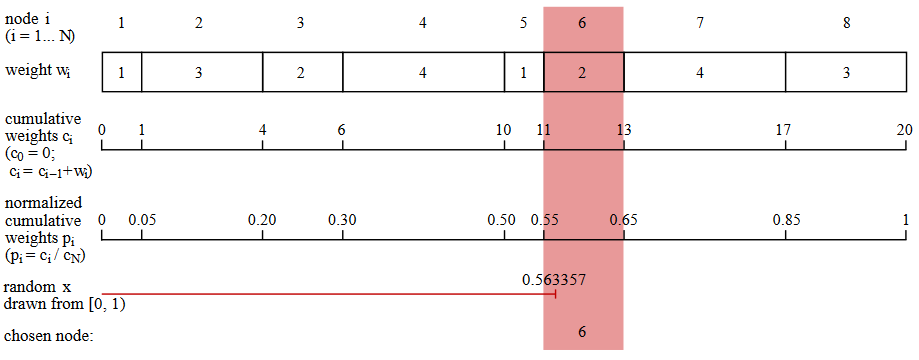
Here is the simplest algorithm I know for random weighted selection. (This is not the most efficient of these algorithms, but better methods are even more chaotic. Keith Schwartz wrote an excellent tutorial and review.on this topic.) Suppose that a data structure that simulates a network node includes a list of links to other nodes and a corresponding list of weights. As shown in the figure below, the program generates a series of accumulated amounts of weights:. The next step is to normalize this series by dividing each number by the total amount of weights. Now we have a series of numbersmonotonically increasing from zero to one. Next, the program selects a random real number from the interval ; must be in one of the normalized intervals and that value determines the next node to select.
In the code in the Julia programming language, the procedure for selecting a node looks like this:
functionselect_next(links, weights)
    total = sum(weights)
    cum_weights = cumsum(weights)
    probabilities = cum_weights / total
    x = rand()
    fori in 1:length(probabilities)
        if probabilities[i] >= x
            returniendendend
I slowly describe these boring details of the accumulated sums and pseudo-random numbers, in order to emphasize in such a way that this algorithm for traversing the graph is not as simple as it looks at first glance. And we still have not considered the topic of probabilities change on the fly, although our attention floats from topic to topic.
It is even more difficult to comprehend the learning process — adding new nodes and edges to the network. I ended my session of free associations when I came to a question I could not answer: how is a butterfly called in Russian? But now I can answer it. Next time when I play this game, I will add babochka to the list . In a computational model, the node insertion for the word babochka- This is a fairly simple task, but our new node should also be connected to all existing nodes about butterflies. Moreover, babochka itself adds new edges. She is phonetically close to babushka (grandmother) - one of several Russian words in my dictionary. The suffix -ochka is diminutive, so you need to associate it with French- itte and Italian- ini . The literal meaning of the word babochka is “little soul,” which implies an even greater number of associations. In the end, the study of a single new word may require a complete reindexing of the entire tree of knowledge.
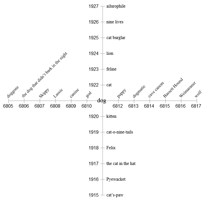
Let's try another method. Forget about accidentally traversing the network with its spaghetti from pointers to nodes. Instead, let's just keep all the similar things in the neighborhood. From the point of view of the banks of the memory of a digital computer, this means that similar things will be stored at adjacent addresses. Here is a hypothetical memory segment centered on the dog concept . Neighboring places are occupied by other words, concepts and categories, which are likely to be caused by the thought of a dog ( dog ): obvious cat (cat) and puppy(puppy), different breeds of dogs and a few specific dogs (Skippy is our family dog, which I had in my childhood), and also, perhaps, more complex associations. Each item has a numeric address. The address does not have any deep meaning, but it is important that all memory cells are numbered in order.
| address | content |
|---|---|
| 19216805 | god |
| 19216806 | the dog that didn't bark in the night |
| 19216807 | Skippy |
| 19216808 | Lassie |
| 19216809 | canine |
| 19216810 | cat |
| 19216811 | dog |
| 19216812 | puppy |
| 19216813 | wolf |
| 19216814 | cave canem |
| 19216815 | Basset hound |
| 19216816 | Weimaraner |
| 19216817 | dogmatic |
The task of leisurely wandering through this array in memory can be quite simple. It can perform a random bypass of memory addresses, but the advantage will be given to small steps. For example, the next visited address may be determined by sampling from the normal distribution centered around the current location. Here is the code for Julia. (The function
randn()returns a random real number obtained from a normal distribution with an average and standard deviation .)functiongaussian_ramble(addr, sigma)
r = randn() * sigma
return addr + round(Int, r)
endSuch a scheme has attractive features. It is not necessary to tabulate all possible target nodes before selecting one of them. Probabilities are not stored as numbers, but are encoded by position in the array, and also modulated by the parameterwhich determines how far the procedure wants to move in the array. Although the program still performs arithmetic to gamble from the normal distribution, such a function is likely to be a simpler solution.
Still, this procedure has a terrifying flaw. Having surrounded the dog with all its immediate associations, we left no room for their associations. Dog terms are good in their own context, but what about the cat in the list? Where do we put kitten , tiger , nine lives and Felix ? In a one-dimensional array, there is no possibility to embed each memory element in a suitable environment.
So let's go in two dimensions! Dividing the addresses into two components, we define two orthogonal axes. The first half of each address becomes a coordinate.and the second is the coordinate . Now dog and cat are still close neighbors, but they also have personal spaces in which they can play with their own "friends."
However, two measurements are not enough either. If we try to fill in all the elements related to The Cat in the Hat , they will inevitably start to clash and conflict with the close elements of the dog that didn't bark in the night . Obviously, we need more dimensions - much more.
Now is the right time to confess - I am not the first to think about how memories can be organized in memory. The list of my predecessors can be begun with Plato, who compared memory with a bird; we recognize the memories by their plumage, but sometimes it is difficult for us to get them if they start to flutter in the cage of our skull. The 16th-century Jesuit Matteo Ricci wrote about the “Palace of Memory”, in which we wander through various rooms and corridors in search of the treasures of the past. Modern theories of memory are usually less figurative, but more detailed and aimed at moving from metaphor to mechanism. Personally, I like the mathematical model obtained in the 1980s by Pentti Kanerva , who now works at the Redwood Center for Theoretical Neurosciences here in Berkeley, most of all . He came up with the ideasparse distributed memory , which I will call SDM. It successfully uses the amazing geometry of high-dimensional spaces.
Imagine a cube in three dimensions. If we assume that the side length is equal to the unit of measurement, then the eight vectors can be denoted by vectors of three binary digits, starting with and ending . At any of the vertices, changing the single bit of the vector brings us to the top, which is the nearest neighbor. Changing two bits moves us to the next nearest neighbor, and replacing all three bits leads to the opposite corner of the cube - to the most distant vertex.
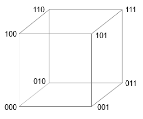
The four-dimensional cube works in a similar way - vertices are indicated by vectors containing all combinations of binary digits starting and ending . This description is actually summarized to measurements where each vertex has -bit vector of coordinates. If we measure the distance along the Manhattan metric - always moving along the edges of the cube and never cutting diagonally - then the distance between any two vectors will be the number of positions in which two coordinate vectors differ (also known as the Hamming distance). (For the exclusive OR, the symbol, sometimes called a bun , is usually used. It displays the XOR operation as a binary modulo-2 addition. Kanerva prefers ∗ or ⊗ on the grounds that the role of XOR in high-dimensional calculations is more like multiplication than addition. I decided to move away from this controversy using the & veebar; - an alternative way to record XOR, familiar in the environment of logicians. This is a modification of ∨ - the symbol of inclusive OR. Conveniently, it is also a XOR symbol in Julia programs.) Thus, the unit for measuring distance is one bit, and calculating the distance is the task for the binary exclusive operator OR (XOR, & veebar;), which gives us the value for different bits, and for the same pairs - the value :
0⊻ 0 = 00⊻ 1 = 11⊻ 0 = 11⊻ 1 = 0The function on Julia to measure the distance between the vertices applies the XOR function to two coordinate vectors and returns the number as a result .
functiondistance(u, v)
    w = u ⊻ v
    return count_ones(w)
end
When becomes large enough some curious properties appear -Cuba. Will consider-dimensional cube having vertices. If you randomly select two of its vertices, then what is the expected distance between them? Although this is a question of distance, we can answer it without delving into geometry - this is just the task of calculating positions in which two binary vectors are distinguished. For random vectors, each bit can be equally likely to be or therefore, it is expected that the vectors will differ in half of the bit positions. When-bit vector standard distance is bats. This result does not surprise us. However, it is worth noting that all distances between the vectors are closely accumulated around the mean value of 500.
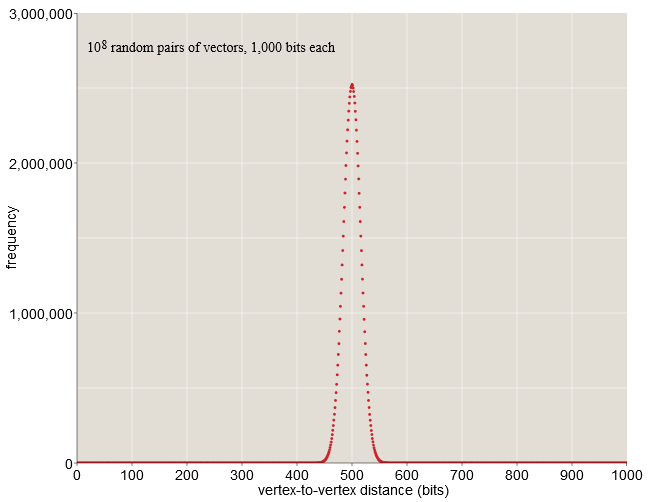
When bit vectors almost all randomly selected pairs are at a distance from before bit. In a sample of one hundred million random pairs (see chart above), none of them are closer than bit or farther than bit. Nothing in our life in a low-resolution space prepared us for such a cluster of probabilities in the middle distance. Here, on Earth, we can find a place in which we will be completely alone, when almost everyone is a few thousand kilometers away from us; however, there is no way to redistribute the world's population in such a way that everyone is in such a state at the same time. But in-dimensional space the situation is as follows.
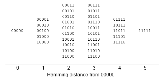
Needless to say, it's hard to imagine-dimensional cube, but we can get a small intuitive understanding of geometry at least on the example of five dimensions. Below is a table of all the coordinates of the vertices in the five-dimensional cube of unit dimension, aligned in accordance with the Hamming distance from the initial point. Most of the peaks (20 of 32) are located at medium distances - two or three bits. The table would have the same shape at any other vertex taken as the starting point.
Serious objection to all these discussions. -dimensional cubes is that we can never build something like this; there are not enough atoms in the universe for the structure ofparts. But Kanerva points out that we need spaces to store only those items that we want to store. We can design equipment for random sampling, for example vertices (each of which has -bit address) and leave the rest of the cube a ghostly, unfinished infrastructure. Kanerva calls such a subset of vertices that exists in the hardware, hard locations . Set ofrandom solid cells will still show the same compressed distance distribution as a full cube; this is exactly what is shown in the graph above.
The relative isolation of each vertex in a high-dimensional cube gives us a hint of one possible advantage of a discharged distributed memory: the stored element has enough space and it can be distributed over a vast area without interfering with its neighbors. This is really an outstanding feature of SDM, but there is something else.
In traditional computer memory, addresses and stored data elements are matched one to one. Addresses are ordinal integers of a fixed range, say. Each integer in this range defines a single individual place in memory, and each place is associated with exactly one address. In addition, only one value is stored in each location at a time; When writing a new value, the old one is overwritten.
SDM violates all of these rules. It has a huge address space - no less- but only a tiny, random share of these places exists as physical entities; this is why memory is called sparse . A single piece of information is not stored in just one memory location; multiple copies distributed over the area - therefore it is distributed. Moreover, in each single address can be stored several data elements. That is, the information is spread over a wide area, and squeezed into one point. This architecture also blurs the distinction between memory addresses and memory contents; in many cases, the stored bit pattern is used as a private address. Finally, the memory may respond to a partial or approximate address and with a high probability of finding the correct item. While traditional memory is an "exact match mechanism," SDM is a "best match mechanism" that returns the element that is most similar to the requested one.
In his 1988 book, Kanerva gives a detailed quantitative analysis of sparse distributed memory with measurements and solid cells. Solid cells are randomly selected from the entire space.possible address vectors. Each solid cell has space to store multiplebit vectors. The memory is generally designed to hold at leastunique patterns. Below, I will consider this memory as a canonical SDM model, despite the fact that it is too small by mammalian standards, and in its newer work, Kanerva focused on vectors with no less thanmeasurements.
This is how memory works in a simple computer implementation. Team
store(X)writes vector memory, considering it both address and content. Value saved to all solid cells that are within a certain distance to . In the canonical model, this distance is 451 bits. It sets the “access circle”, designed to combine approximatelysolid cells; in other words, each vector is stored approximately inout of a million solid cells. It is also important to note that the stored item not necessary to choose from binary vectors that are addresses of solid cells. On the contrary. can be any of possible binary patterns.
Suppose a thousand copies are already recorded in SDMfollowed by a new item , which also needs to be saved in its own set of thousands of solid cells. There can be intersection between these two sets - the places where they are stored andand . The new value does not overwrite or replace the previous one; both values are preserved. When the memory fills up to its capacity ineach of them saved times, and in a typical solid cell will be stored copies unique patterns.
Now the question is this: how can we use this mixed memory? In particular, how do we get the right valuewithout affecting and all the other items that have accumulated in one storage place?
The read algorithm will use the property of a curious distribution of distances in a high dimensional space. Even and are the nearest neighbors of stored patterns, they are likely to differ by 420 or 430 bits; therefore, the number of solid cells in which both values are stored is small enough — usually four, five, or six. The same applies to all other patterns intersecting with. There are thousands of them, but none of the affecting patterns are present in more than a few copies within the access circle..
The command
fetch(X)must return the value previously written by the command store(X). The first step in recreating the value is to collect all the information stored within the 451-bit access circle centered on. Insofar as was previously recorded in all these places, we can be sure that we will get his copies. We will also get aroundcopies of other vectors stored in places where access circles intersect with circles. But since the intersections are small, each of these vectors is present in only a few copies. Then in general, each of them bit equiprobably can be or . If we apply the majority principle function to all the data collected in each bit position, then the result will be dominated copies . Probability of getting different from result is approximately equal to . The majority principle procedure is shown in more detail below on a small example of five data vectors of 20 bits each. The output will be a different vector, each bit of which reflects the majority of the corresponding bits in the data vectors. (If the number of data vectors is even, then “draws” are resolved by randomly selecting or .) The alternative writing and reading scheme shown below refuses to store all patterns separately. Instead, it stores the total number of bits. and in every position. Solid cell has-bit counter, initialized by all zeros. When writing a pattern into place, each bit counter is incremented for or decreases for . The read algorithm simply looks at the sign of each bit counter, returning for a positive value, for a negative and random value when the counter bit is .

These two storage schemes give identical results.
From the point of view of computing, this version of sparse distributed memory looks like an elaborate joke. To memorizeelements we need a million solid cells in which we will store a thousand redundant copies of each pattern. To extract only one item from memory, we collect data onsaved patterns and use for disentangling the mechanism of the principle of majority. And all this is done with the help of a heap of acrobatic maneuvers just to get the vector, which we already have. Traditional memory works much less erratically: both writing and reading access one place.
But SDM can do what traditional memory is incapable of. In particular, it can extract information based on partial or approximate data. Let's say a vector is a damaged version in which have changed of vectors. Since the two vectors are similar, the team
fetch(Z)will visit many of the same places where they are stored. With a Hamming distance of 100, we can expect and about 300 solid cells will be common. Thanks to this large intersection, the vector returned is fetch(Z)(let's call it) will be closer to what is . Now we can repeat this process with a team fetch(Z′)that will return the result.even closer to . In just a few iterations, the procedure will reach. Kanerva showed that the convergent sequence of recursive read operations will lead to success with almost complete certainty if the initial pattern is not too far from the target pattern. In other words, there is a critical radius: any test of memory, starting from a spot inside the critical circle, will almost exactly converge to the center, and will do it fairly quickly. Attempting to restore an item stored outside the critical circle will fail, because the recursive recall process will move away by an average distance. The Kanerva analysis showed that for a canonical SDM, the critical radius is 209 bits. In other words, if we know about 80 percent of the bits, then we can recreate the entire pattern.
In the illustration below, the evolution of sequences of recursive memories is monitored using source signals that differ from the target on . In this experiment, all sequences starting at a distance or less converge to behind or less iterations (blue traces) . All sequences starting at a larger initial distance wander aimlessly through vast empty spaces.-dimensional cube, remaining approximately 500 bits from any place.
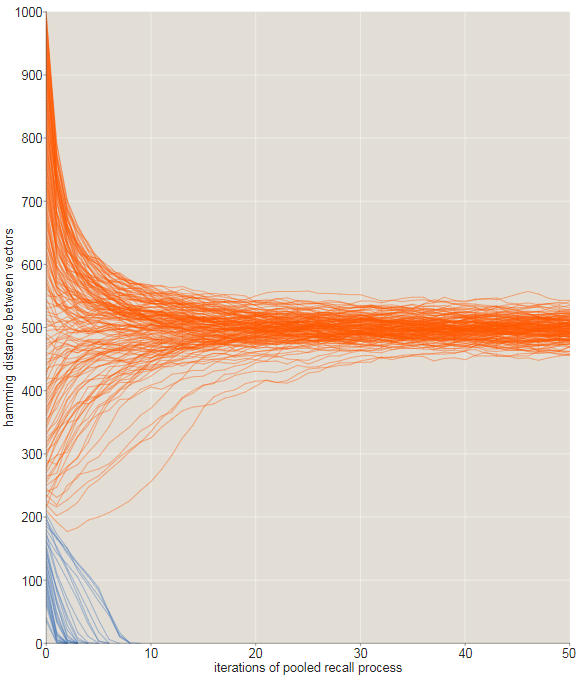
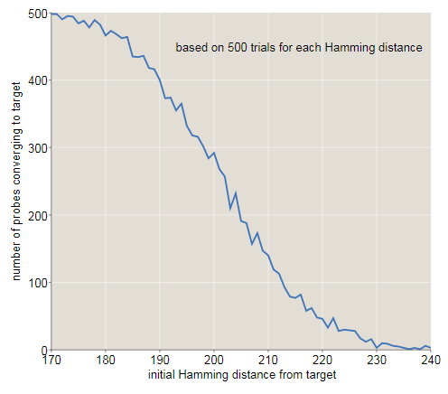
The transition from converging to diverging trajectories is not ideal rosaries, and this is noticeable in the tattered graph shown below. Here we zoomed in to look at the fate of the trajectories starting with offsets inbit. All starting points that are within 209 bits from the target are indicated in blue; those starting from longer distances are orange. Most of the blue paths converge, quickly moving to zero distance, and most orange - no. However, close to the critical distance there are many exceptions.

The graph below shows another look at how the original distance from the target affects the probability of descending to the correct memory address. With a distance ofbit of success almost all attempts end; atalmost all are unsuccessful. It seems that the intersection point (at which success and failure are equally likely) lies approximately in bits, slightly lower than the Kanerva result, equal to . (There is nothing mysterious in this discrepancy. In Kanerva’s calculations, the access circle is assumed to be limiting exactlysolid cells. My experiments included all solid cells within a distance.; on average there such places.)
The ability to recreate memories from partial information is a familiar element of human life. You notice an actor in a television show, and understand that you have seen him before, but you do not remember where. In a few minutes you reach: this is Mr. Bates from Downton Abbey , but without a butler costume. High school graduates meeting: looking at the tight, balding gentleman on the other side of the room, can you find out in him a friend who was only known as a teenager in sport shorts? Sometimes long efforts are required to fill the gaps. I already wrote about my own inexplicable "blind spot" in memory of growing wisteria, which I could call only after patiently flipping through the catalog of fake smells: hydrangeas, verbena, forsythia.
Can our ability to recover memories from incomplete or noisy input data work like a recursive process of recalling high-dimensional vectors? This would be an attractive hypothesis, but there are reasons to be wary of it. For example, the brain seems to be able to extract meaning from much more scarce signals. I do not need to listen to four fifths of the “Fifth Symphony” in order to identify it, the first four notes are enough. The color flashed through the trees instantly makes you remember the corresponding bird species — the cardinal, the blue jay, and the squirrel. The slightest whiff of chalk dust brings me back to the sleepy, sultry class in which I drew half a day at the desk. Such memories are caused by tiny fractions of the information representing them, far less than 80 percent.
Kanerva mentions another feature of human memory that can be modeled with the help of SDM: the phenomenon “spins on the tip of the tongue”, the essence of which is that you know that you know something, although you cannot immediately call it. This feeling is quite mysterious: if you cannot find what you were looking for, how can you know that it is all stored in the brain? The recursive recall process from SDM offers us a possible answer. When successive patterns taken from memory become constantly closer to each other, we can reasonably be sure that they will converge to the goal even before they get to it.
In trying to extract stubborn fact from memory, many people find that constantly knocking on the same door is not the wisest strategy. Instead of demanding immediate answers - to command your brain - it is often better to put the task aside, take a walk, perhaps take a nap; the answer may come as if he were uninvited. Can this observation be explained by the SDM model? Perhaps at least partially. If the sequence of recalled patterns does not converge, then further investigation of it may turn out to be fruitless. If you start again from a neighboring point in the memory space, you can come to a better result. But there is a mystery: how to find a new starting point with better prospects? You might think that it’s enough just to randomly replace a few bits in the input pattern and hope as a result, he will be closer to the goal, but the probability of this is small. If the vector is in bits from the target then bits already true (but we do not know any ofbit); with any random change we have a probability indo not come close, and go even further. To make progress, you need to know in which direction to move, and in-dimensional space is a difficult question.
One aspect of the SDM architecture is that it seems to have a repetitive or repeated listening effect on the memory. If you repeat a poem several times or practice a musical work, you can expect that in the future you will remember it more easily. The computational model should demonstrate a similar training effect. But in traditional computer memory this is impossible: there are no advantages in rewriting the same value several times at the same address. In SDM, on the contrary, each repetition of a pattern adds another copy to all solid cells within the pattern's access circle. As a result, there is less influence from intersecting patterns, and the critical radius of recall increases. The effect has a significant effect: bit up more than .
Similarly, playing one pattern can make it difficult to restore the rest. This is reminiscent of forgetting, when an actively sealed pattern fills its neighbors and captures part of their territory. This effect also has a significant effect on SDM, so much so that it even seems unreal. It seems that a vector saved eight or ten times monopolizes most of the memory; he becomes an obsession, the answer to all questions.
An important advantage of sparse distributed memory is its resistance to hardware failures or errors. I would be upset if the loss of a single neuron in my brain left a hole in my memory, and I could not recognize the letter gor remember how to tie shoelaces. SDM does not suffer from such fragility. When each stored pattern has a thousand copies, no place is important. And in fact, you can erase all the information stored in 60 percent of the solid cells, and still have the perfect memory., if we assume that we are transmitting an absolutely exact address as a signal. With partial signals, the critical radius is compressed as the number of lost points increases. After the destruction of 60 percent of the sites, the critical radius is compressed with bit up to about bit. After the destruction of 80 percent of the places the memory is seriously damaged, but not destroyed.
What about wandering in the clouds? Can we idly wander through the meadows of sparse distributed memory, by luck by jumping from one stored pattern to another? I will return to this issue.
Most of the above was written a few weeks ago. At that time, I read about various competing theories of memory and discussed their virtues with colleagues from the Simons Institute. I wrote down my thoughts on this topic, but I postponed their publication due to persistent doubts: did I understand the mathematics of sparse distributed memory correctly? Now I am glad that I was in no hurry.
The program "Brain and Calculations" was completed in May. Its members dispersed: I returned to New England, where sage and rosemary are small potted plants, and not lush bushes hanging over the paths. My morning walks to the campus at Berkeley, daily opportunities to reflect on the nature of memory and learning, became “engrams” stored somewhere in my head (however, I still don’t know where to find them).
However, I did not give up my searches. After leaving Berkeley, I continued to read about theories of memory. I also wrote programs for studying the sparse distributed memory of Pentti Kanerva and his more extensive ideas of “hyperspace computing”. Even if this project fails to reveal to me the secrets of human memory, it will definitely teach me something about the mathematical and computational art of navigation in high-dimensional spaces.
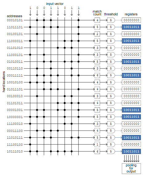
The diagram below shows the “right” way to implement SDM, as I understand it. The main element is a cross matrix in which the rows correspond to solid memory cells, and the columns carry signals that simulate individual bits of the input vector. There are a million lines in canonical memory, each of which is randomly assigned-bit address, and columns; This demo version consists of 20 rows and 8 columns.
The process illustrated in the diagram is to save one input vector to empty memory. The eight input bits are simultaneously compared with all 20 addresses of solid cells. When the input bit and address bit match — zero with zero or one with one — we put a period at the intersection of the column and row. Then we count the number of points in each line, and if the number is equal to or exceeds the threshold value, then we write the input vector to the register associated with this line (blue fields) . In our example, the threshold value is 5, and in 8 out of 20 addresses there are at least 5 matches. AT-bit memory threshold value will be equal to , and selected will be only about one-thousandth of all registers.
The magic of this architecture is that all bit comparisons — and a billion in the canonical model — occur simultaneously. Therefore, the access time for reading and writing does not depend on the number of solid cells and can be very small. This generic layout, known as associative memory or content-addressable memory, is used in some computing areas, such as turning on particle detectors in the Large Hadron Collider and transmitting packets through routers on the Internet. And the circuit diagram can be associated with certain brain structures. Kanerva indicates that the cerebellum is very similar to this matrix. The rows are flat, fan-shaped Purkinje cells, assembled like book pages; the columns are parallel fibers stretching across all Purkinje cells. (However, the cerebellum is not a region of the mammalian brain,
It would be great to build an SDM simulation based on this cross-architecture; Unfortunately, I do not know how to implement it on the computer equipment I have at my disposal. In a traditional processor, there are no ways to simultaneously compare all input bits with bits of solid cells. Instead, I have to go through a million solid cells in succession, and compare thousands of bits in each place. This represents a million bit comparisons for each item stored or retrieved from memory. Add to this the time to write or read a million bits (thousands of copies-bit vector), and you have a rather slow process. Here is the code to save the vector:
functionstore(v::BitVector)for loc in SDM
        if hamming_distance(v, loc.address) <= r
            write_to_register!(loc.register, v)
         endendend
This implementation takes about an hour to inventory memory with memorized patterns. (The complete program in the form of Jupyter notebook is laid out on GitHub .)
Is there a better algorithm for simulating SDM on a regular hardware? One of the possible strategies allows avoiding a repetitive search for a set of solid cells within the access circle of a given vector; instead, when the vector is first written to memory, the program stores a pointer to each of the thousands or so of the places in which it is stored. In the future, with any reference to the same vector, the program can proceed bysaved pointers, rather than scanning the entire array of a million solid cells. The price of this caching scheme is the need to store all these pointers — in canonical SDM themmillion This is very realistic, and can be worth it if you want to store and retrieve only accurate, known values. But think about what happens in response to an approximate memory request with recursive recall. and and , and so on. None of these intermediate values will be found in the cache, so you still need a full scan of all solid cells.
Perhaps there is a more tricky opportunity to cut the path. Alexander Andoni, Peter Indyk and Ilya Razenshteyn, a recent review article on Approximate Nearest Search and High Dimensions , mentions an intriguing technique called locality sensitive hashing, but for the time being I don’t quite understand how to adapt it to the SDM task.
The ability to restore memories from partial signals is a painfully human feature of the computational model. Perhaps it can be expanded to obtain a plausible mechanism for idle wandering around the halls of the mind, in which one thought leads to the next.
At first I thought I knew how this could work. Pattern stored in SDM creates around itself a region of attraction in which any recursive study of memory, starting from a critical radius, converges to . WithWith such attractors, I can imagine how they divide the memory space into a matrix of individual modules like high-sized foam bubbles. The area for each stored element occupies a separate volume, surrounded on all sides by other areas and resting against them, with clear boundaries between adjacent domains. In support of this judgment, I can see that the average radius of the region of attraction, when new content is added to the memory, shrinks, as if the bubbles were shrinking due to overcrowding.
Such a vision of the processes inside the SDM implies a simple way to move from one domain to another: you need to randomly switch enough bits of the vector to move it from within the current region of attraction to the next, and then apply the recursive recall algorithm. Repeating this procedure will generate a random crawl of multiple themes stored in memory.
The only problem is that this approach does not work. If you check it, then he really will aimlessly wander aroundlattice, but we will never find anything stored there. The entire plan is based on an erroneous, intuitive understanding of SDM geometry. Stored vectors with their regions of attraction are not packed tightly like soap bubbles; on the contrary, they are isolated galaxies hanging in a vast and free universe, separated by vast stretches of empty space between them. Brief calculations show us the true nature of the situation. In the canonical model, the critical radius determining the region of attraction is approximately equal to. The volume of a single area, measured as the number of vectors inside, is equal to
which is about equal . Therefore, all areas occupy volume . This is a large number, but it’s still a tiny fraction.-dimensional cube. Among all the vertices of the cube only of lies within 200 bits of the saved pattern. You can always wander, and not stumbled upon any of these areas.
(Eternally? Oh, well, yes, maybe not forever. Since the hypercube is a finite structure, any way through it sooner or later must become periodic, or if it hits a fixed point that it never leaves, or gets lost in a repeating cycle The stored vectors are fixed points, in addition, there are many other fixed points that do not correspond to any meaningful pattern. Be that as it may, in all my experiments with SDM programs I have never been able to “accidentally” get into a saved pat turn)
Trying to save this unfortunate idea, I conducted a few more experiments. In one case, I arbitrarily saved several related concepts to neighboring addresses ("neighboring", that is
, within 200 or 300 bits). Perhaps, within this cluster, I can carelessly jump from point to point. But in reality, the entire cluster is condensed into one large area of attraction for the central pattern, which becomes a black hole, sucking in all its companions. I also tried to play around with the value(access circle radius for all read and write operations). In the canonical model. I thought that writing to a slightly smaller circle or reading from a slightly larger circle would leave enough space for randomness in the results, but this hope did not come true either.
All these attempts were based on the misunderstanding of high-dimensional vector spaces. An attempt to find clusters of neighboring values in a hypercube is hopeless; stored patterns are too far apart. Arbitrary creation of dense clusters is also meaningless, because it destroys the very property that makes the system interesting - the ability to converge to the stored element from anywhere in the surrounding area of attraction. If we want to create an algorithm for wandering in the clouds for SDM, then we need to come up with some other way.
In search of an alternative mechanism for the flow of consciousness, you can try to add a little graph theory to the world of sparse distributed memory. Then we can take a step back, back to the original idea of mental walks in the form of a random walk around a graph or network. The key element for embedding such graphs in SDM turns out to be a familiar tool: the exclusive OR operator.
As stated above, the Hamming distance between two vectors is calculated by taking their bitwise XOR and calculating the resulting result of units. But the XOR operation gives not just the distance between two vectors, but also other information; it also determines the orientation or direction of the line connecting them. In particular, the operation gives a vector listing the bits that need to be changed to convert at and vice versa. Can also be perceived and in the XOR vector as a sequence of directions to follow to track the path from before .
XOR has always been my favorite of all boolean functions. This is a difference operator, but unlike subtraction, XOR is symmetric:. Moreover, XOR is its own inverse function. This concept is easy to understand with functions with a single argument: is a proper inverse function if , that is, after applying the function twice, we can go back to where we started. For a function with two arguments, such as XOR, the situation is more complicated, but it is still true that performing the same action twice restores the original state. In particular, ifthen and . Three vectors -, and - create a tiny closed universe. For any pair of them, you can apply the XOR operator and get the third element of the set. Below is my attempt to illustrate this idea. Each square imitates-bit vector lined up as a 100 x 100 table of light and dark pixels. Three patterns seem random and independent, but in reality each panel is the XOR of the other two. For example, in the leftmost square, each red pixel corresponds either to green or blue, but never to both.
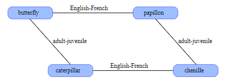
The self-inverting property tells us a new way of organizing information in SDM. For example, the word butterfly and its French analogue papillon are stored in arbitrary, random vectors. They will not be close to each other; the distance between them is likely to be approximately equal to 500 bits. Now we compute the XOR of these vectors butterflypapillon ; the result is another vector that can also be saved in SDM. This new vector encodes the link English-French . Now we have a translation tool. Having a vector for a butterfly , we perform an XOR for it with an English-French vector and get a papillon . The same trick works in the opposite direction.
This pair of words and the connection between them form the core of the semantic network. Let's increase it a little. We can save the word caterpillar in an arbitrary address , and then calculate the butterflycaterpillar and name this new adult-junior relationship . What is the French name for caterpillar ? The caterpillar in French is chenille . We add this fact to the network, keeping chenille at caterpillarEnglish-French . Now is the time of magic: if we take papillonchenille , then we learn that these words are related by the adult-young ratio , even though they did not explicitly indicate this. This restriction is imposed by the geometry of the structure itself.
The graph can be expanded further by adding more Anglo-French related words ( dog-chien, horse-cheval ) or more adult-young pairs: ( dog-puppy, tree-sapling ). You can also explore many other links: synonyms, antonyms, siblings, cause and effect, predator-prey, and so on. There is also a great way to connect multiple events into a chronological sequence by simply performing XOR for the predecessor and follower addresses.
The way to connect concepts through XOR is a hybrid of geometry and graph theory. In the mathematical theory of ordinary graphs, distances and directions are irrelevant; the only thing that matters is the presence or absence of connecting edges between nodes. On the other hand, in SDM, the edge-representing link between nodes is a vector of finite length and directivity in-dimensional space. For a given node and link, the XOR operation “binds” this node to a specific position somewhere else in the hypercube. The resulting structure is absolutely rigid - we cannot move a node without changing all the links in which it participates. In the case of butterflies and caterpillars, the configuration of the four nodes inevitably turns out to be a parallelogram, where the pairs on opposite sides have the same length and direction.
Another unique characteristic of an XOR-related graph is that nodes and edges have exactly the same representation. In most computer implementations of ideas from graph theory, these two entities are very different; a node can be a list of attributes, and an edge can be a pair of pointers to the nodes it connects. In SDM, both nodes and edges are simply high-dimensional vectors that can be stored in the same format.
When used as a human memory model, the XOR binding allows us to connect any two concepts through any connection we can come up with. The multitude of connections in the real world is asymmetrical; they do not have the self-inverting property that XOR has. The XOR vector may declare that Edward and Victoria are the parent and child, but do not indicate which of them is who. Worse, the XOR vector connects exactly two nodes and never again, so the parent of several children puts us in an unpleasant position. Another difficulty lies in maintaining the integrity of all branches of a large graph with each other. We cannot simply add nodes and edges arbitrarily; they must be attached to the graph in the correct order. Inserting the pupal stage between the butterfly and the caterpillar will require rewriting most of the scheme;
Some of these problems are solved in another XOR-based technique, which Kanerva calls bundling. The idea is to create a database for storing attribute-value pairs. An entry for a book can have attributes such as author , title, and publishereach of which is paired with a corresponding value. The first stage of data banding consists of a separate XOR for each attribute-value pair. Then the vectors derived from these operations are combined to create a single total vector using the same algorithm described above for storing several vectors in a solid SDM cell. By performing an XOR attribute name with this combined vector, we get an approximation of the corresponding value, close enough to be determined by the method of recursive recall. In experiments with the canonical model, I found out that-bit vector can store six or seven attribute-value pairs without much risk of confusion.
Binding and banding are not mentioned in the Kanerva book of 1988, but he tells in detail about them in newer articles. (See the “Additional Reading” section below.) It indicates that with these two operators, the set of high-dimensional vectors acquires the structure of an algebraic field, or at least an approximation to a field. The canonical example of a field is the set of real numbers instead of with the operations of addition and multiplication, as well as their inverse operators. Real numbers create a closed set for these operations: the addition, subtraction, multiplication or division of any two real numbers gives another real number (except for division by zero, which is always a joker in the deck). Similarly, the set of binary vectors is closed for linking and banding, except
Can tying and banding help us in getting a soaring algorithm in the clouds? They provide us with basic tools for navigating a semantic graph, including the ability to perform a random walk. Starting from any node in a connected XOR graph, the random crawl algorithm chooses among all the links present in this one. Randomly choosing a communication vector and performing XOR of this vector with the node address leads us to another node, where the procedure can be repeated. Similarly, in attribute-value pairs of a bundling, a randomly selected attribute triggers the corresponding value, which becomes the next node under investigation.
But how does the algorithm know which links or which algorithms are available for selection? Links and attributes are presented in the form of vectors and stored in memory like any other objects, so there are no obvious ways to get these vectors, unless you know what they really are. We cannot tell the memory "show me all the connections." We can only show the pattern and ask “is there such a vector? Did you see something like that? ”
In a traditional computer memory, we can get a memory dump: go through all the addresses and output the value found in each place. But for distributed memory there is no such procedure. To me this depressing fact was given with difficulty. When building a computational model SDM, I managed to achieve a good enough work to be able to store in memory several thousand randomly generated patterns. But I could not retrieve them, because I did not know what to request. The solution was to create a separate list outside of the SDM itself, in which everything that I save would be written. But the assumption that the brain would store both the memory and the index of this memory seems far-fetched. Why not just use the index, because it is much easier?
Due to this limitation, it appears that sparse distributed memory is equipped to serve the senses, but not the imagination. She can recognize familiar patterns and save new ones that will be recognized in subsequent meetings, even from partial or damaged signals. Thanks to linking or banding, memory can also track connections between pairs of stored items. But everything that is written into memory can only be retrieved by transmitting a suitable signal.
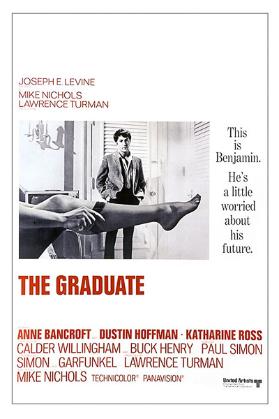
When I look at the Graduate poster , I see Dustin Hoffman looking at Ann Bancroft's leg in a stocking. This visual stimulus excites a subset of neurons in the cerebral cortex, corresponding to my memories of the actors, characters, plot, soundtrack, and 1967. All of this brain activity can be explained by the SDM memory architecture, if we assume that the subsets of neurons can be represented in some abstract form as long random binary vectors. But it is impossible to just as simply explain that I can cause all the same sensations in my brain without seeing this picture. How do I specifically extract these long random sequences from a huge interweaving of vectors, not knowing exactly where they are?
This is where my long journey ends - a note of doubt and frustration. It hardly surprises you that I was not able to get to the bottom line. This is a very difficult topic.
On the very first day of the “Brain and Computing” program at the Simons Institute, Jeff Lichtman, who is working on tracing the switching circuit in the brain of mice, asked the question: have neuroscience reached Watson-Creek moment? In molecular genetics, we have reached the point where we were able to heal a DNA chain from a living cell and count many of the messages in it. We can even record our own messages and insert them back into the body. A similar ability in neuroscience would be the study of brain tissue and the reading of information stored in it - knowledge, memories, and world views. Perhaps we could even record information directly to the brain.
Science has not even come close to achieving this goal, to the joy of many. Including me: I do not want my thoughts to be sucked out of my head through electrodes or pipettes and replaced with #fakenews. However, I really want to know how the brain works.
The Simons Institute program blinded me with the recent successes of neuroscience, but also made me understand that one of the most serious questions remains unanswered. The projects of Likhtmann and others on connectomics create a detailed map of the millions of neurons and their connections. New recording techniques allow us to listen to the signals emitted by individual neurocytes and follow the excitation waves over wide areas of the brain. We have a fairly comprehensive catalog of neuron types and we know a lot about their physiology and biochemistry. All this is impressive, but there are still riddles. We can record neural signals, but for the most part we do not know what they mean. We do not know how information is encoded and stored in the brain. This is like trying to understand a digital computer's circuit diagram without knowing binary arithmetic and Boolean logic.
The Pentti Kanerva Sparse Distributed Memory Model is one attempt to fill in some of these gaps. This is not the only such attempt. A more well-known alternative is the approach of John Hopfield - the concept of a neural network as a dynamic system that takes the form of an energy minimizing attractor. These two ideas have common basic principles: information is scattered over a huge number of neurons and is encoded in a form that is not obvious to an external observer, even he will have access to all neurons and signals passing through them. Such schemes, which are essentially mathematical and computational, are conceptually located in the middle between high-level psychology and low-level neural engineering. In this layer is the value.
Additional reading
Hopfield, J. J. (1982). Neural networks and physical systems with emergent collective computational abilities. Proceedings of the National Academy of Sciences 79(8):2554–2558.
Kanerva, Pentti. 1988. Sparse Distributed Memory. Cambridge, Mass.: MIT Press.
Kanerva, Pentti. 1996. Binary spatter-coding of ordered K-tuples. In C. von der Malsburg, W. von Seelen, J. C. Vorbruggen and B. Sendhoff, eds. Artificial Neural Networks—ICANN 96 Proceedings, pp. 869–873. Berlin: Springer.
Kanerva, Pentti. 2000. Large patterns make great symbols: An example of learning from example. In S. Wermter and R. Sun, eds. Hybrid Neural Systems, pp. 194–203. Heidelberg: Springer. PDF
Kanerva, Pentti. 2009. Hyperdimensional computing: An introduction to computing in distributed representation with high-dimensional random vectors. Cognitive Computation 1(2):139–159. PDF
Kanerva, Pentti. 2010. What we mean when we say “What’s the Dollar of Mexico?”: Prototypes and mapping in concept space. Report FS-10-08-006, AAAI Fall Symposium on Quantum Informatics for Cognitive, Social, and Semantic Processes. PDF
Kanerva, Pentti. 2014. Computing with 10,000-bit words. Fifty-second Annual Allerton Conference, University of Illinois at Urbana-Champagne, October 2014. PDF
Plate, Tony. 1995. Holographic reduced representations. IEEE Transactions on Neural Networks 6(3):623–641. PDF
Plate, Tony A. 2003. Holographic Reduced Representation: Distributed Representation of Cognitive Structure. Stanford, CA: CSLI Publications.