Visualization for music player
The information in the article will cover the topic of creating visualizations for a music player. It so happened that the program was written in as3, because this is the language I'm programming in now.
It all started from the Phthalo's Corona visualization seen in the AIMP player . I thought for a long time how it works and finally came up with something. The first prototype was written in C ++. As a result, I only got a prototype of the movement of particles as in this visualization. On this I stopped and after half a year I wanted to work with sound again. After 2 days, such a flash drive was ready. LINK Mouse click - change the blur mode.

In order for it to work correctly, you need to open some kind of music player (for example, on VKontakte) in the browser, and close all the extra tabs with audio data, because when receiving spectral data, through the SoundMixer.computeSpectrum flash drive may crash due to the fact that other applications do not allow you to take audio data from them. If it does not fall, then nothing can be closed. As was noted, in my chrome sound from other tabs is not caught.
Now let's move on to an overview of how this all works.
Particles are located in the region (in this case, 650). 600 active particles and 50 particles that appear at a random point in the region and fall down, when such a particle touches the floor, it will re-respawn in the region. Of course, gravity acts on all particles.
In addition to gravity, particles can be influenced by an attractor and repulsor. Now I will explain what kind of things are so magical. In fact, they are not magical at all, they just have the same abstruse names as any "professors" like to express themselves.
An attractor is such a thing that attracts everything that is possible to itself. In this case, the particles, and the farther the particle is from the attractor, the weaker it is attracted.
A repulsor is the same as an attractor, but on the contrary it repels everything from itself.
So, under certain conditions (based on the sound spectrum), an attractor and a repulsor act on particles. Because of this, they are so jumping in the area.
Bitmapdata is created for particles, one for all (this is logical). This is a small white circle, why white will explain below.
Particles are drawn like this:
The matrix transforms the particles so that they stretch when moving. Nothing complicated.
When starting the visualization, palettes are created from which the color is sampled when rendering the final image (standard fixture of democoders :)
They are randomly selected during operation.
To work with the palette, you need to prepare 3 arrays with a size of 256 values. These will be arrays for red, green and blue.
In order to use them, you must use the paletteMap function of the BitmapData class. It receives these arrays and the original image as parameters.
It works like this:
Now I will explain why the particles must be painted white and the background black.
When applying the filter bloom, all pixels will be blurred and as a result, if you do not draw anything, they will turn black. When applying the palette, black is replaced with any color, so when blurring, the color will smoothly transition to the color we need (in the buffer in which the particles are drawn, the background will remain black).
The palette is constructed so that in the upper indices (255 - white) rgb arrays, the color of the particles is recorded, and in the lower (0 - black) the background color. In all other indices [1..254], gradient colors from the background color to the particle color are recorded. Of course, no one bothers to add more than 2 colors to the palette and make a gradient between them.
In the original visualization, a very interesting twist of the particle trail is made. I peered at him for a long time to understand how it works.
In the end, I came to the conclusion that this is a hyperbolic spiral .
Hyperbolic spiral equation (in polar coordinates):
r * phi = a, where a is the spiral divergence rate
In Cartesian coordinates:
x = a * cos (phi) / phi,
y = a * sin (phi) / phi, where a / phi = r
The question arose of how now to do this O_O. Firstly, you need to somehow set the formula for such a distortion, and secondly how to do it on a flash.
Of course, at first I tried to do everything the old fashioned way, going through all the pixels of the image and shifting the pixels in certain directions, moreover, this would immediately put the blur there. But in practice, everything turned out to be much different. The cycle in the image killed fps. I had to look for another solution.
The idea came up to make a twirl effect, I immediately found the code through DisplacementMapFilter. But this was not what was in the original.
Had to return to the review of the hyperbolic spiral. The whole difficulty was that the spiral is clearly defined through the angle and radius in polar coordinates, and I needed to add another parameter - the thickness. As a result, after deriving some formulas, I wrote an algorithm for generating a displacement map.
The displacement map is constructed according to this algorithm:
Going through all the pixels of the image, each pixel is checked for a spiral (given the thickness). If the pixel belongs to a spiral, then at this point it is necessary to calculate the offset.
To find the direction of displacement, you can take the tangent at a given point. To simplify the calculations, I decided to find the tangent to the circle at a given point. With this approach, the calculation error will be noticeable only in the tail of the spiral. Because as the radius (or angle) y increases, the coordinate tends to a, i.e. to the line.
f '(x, y) = ArcTan (y / x) - Pi / 2
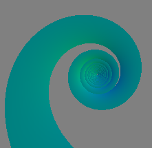
Now just find the vector by the obtained angle and multiply it by the offset coefficient. As a result, we got such a displacement map (green and blue channels are used)
In the second mode, another displacement map is superimposed which is generated by Perlin noise.
Here is such a nice image that is obtained at the output:

It would be possible to add more octaves during generation, but noise is generated every update (for this the octave shift is used, for the motion effect).
As a result, the rendering steps are as follows:
SOURCES .
That's all, thanks for watching!
It all started from the Phthalo's Corona visualization seen in the AIMP player . I thought for a long time how it works and finally came up with something. The first prototype was written in C ++. As a result, I only got a prototype of the movement of particles as in this visualization. On this I stopped and after half a year I wanted to work with sound again. After 2 days, such a flash drive was ready. LINK Mouse click - change the blur mode.
In order for it to work correctly, you need to open some kind of music player (for example, on VKontakte) in the browser, and close all the extra tabs with audio data, because when receiving spectral data, through the SoundMixer.computeSpectrum flash drive may crash due to the fact that other applications do not allow you to take audio data from them. If it does not fall, then nothing can be closed. As was noted, in my chrome sound from other tabs is not caught.
Now let's move on to an overview of how this all works.
Physics
Particles are located in the region (in this case, 650). 600 active particles and 50 particles that appear at a random point in the region and fall down, when such a particle touches the floor, it will re-respawn in the region. Of course, gravity acts on all particles.
In addition to gravity, particles can be influenced by an attractor and repulsor. Now I will explain what kind of things are so magical. In fact, they are not magical at all, they just have the same abstruse names as any "professors" like to express themselves.
An attractor is such a thing that attracts everything that is possible to itself. In this case, the particles, and the farther the particle is from the attractor, the weaker it is attracted.
A repulsor is the same as an attractor, but on the contrary it repels everything from itself.
So, under certain conditions (based on the sound spectrum), an attractor and a repulsor act on particles. Because of this, they are so jumping in the area.
Drawing
Bitmapdata is created for particles, one for all (this is logical). This is a small white circle, why white will explain below.
var radius: Number = PARTICLE_SIZE * 0.5;
var particleShape: Shape = new Shape();
particleShape.graphics.beginFill(0xFFFFFF);
particleShape.graphics.drawCircle(PARTICLE_SIZE * 0.5, PARTICLE_SIZE * 0.5, radius);
m_ParticleBmp = new BitmapData(PARTICLE_SIZE, PARTICLE_SIZE, true, 0x0);
m_ParticleBmp.draw(particleShape);
Particles are drawn like this:
var velDir: Number = Math.atan2(part.vel.y, part.vel.x);
var speed: Number = Math.max(Math.abs(part.vel.y), Math.abs(part.vel.x));
if (speed > 20)
    speed = 20;
matr.identity();
matr.scale(1.3 + speed / 20.0 * 4.0, 0.5);
matr.rotate(velDir);
matr.translate(part.pos.x, part.pos.y);
m_BackBuffer.draw(m_ParticleBmp, matr);
The matrix transforms the particles so that they stretch when moving. Nothing complicated.
Effects
Palette
When starting the visualization, palettes are created from which the color is sampled when rendering the final image (standard fixture of democoders :)
They are randomly selected during operation.
To work with the palette, you need to prepare 3 arrays with a size of 256 values. These will be arrays for red, green and blue.
In order to use them, you must use the paletteMap function of the BitmapData class. It receives these arrays and the original image as parameters.
It works like this:
- the pixel color is taken from the original image, integer;
- this color is broken into rgb (byte) components;
- for these components, the value from the corresponding array is taken, these will be the new rgb values;
- new rgb values are collected back into integer.
Now I will explain why the particles must be painted white and the background black.
When applying the filter bloom, all pixels will be blurred and as a result, if you do not draw anything, they will turn black. When applying the palette, black is replaced with any color, so when blurring, the color will smoothly transition to the color we need (in the buffer in which the particles are drawn, the background will remain black).
The palette is constructed so that in the upper indices (255 - white) rgb arrays, the color of the particles is recorded, and in the lower (0 - black) the background color. In all other indices [1..254], gradient colors from the background color to the particle color are recorded. Of course, no one bothers to add more than 2 colors to the palette and make a gradient between them.
Distortion map
In the original visualization, a very interesting twist of the particle trail is made. I peered at him for a long time to understand how it works.
In the end, I came to the conclusion that this is a hyperbolic spiral .
Hyperbolic spiral equation (in polar coordinates):
r * phi = a, where a is the spiral divergence rate
In Cartesian coordinates:
x = a * cos (phi) / phi,
y = a * sin (phi) / phi, where a / phi = r
The question arose of how now to do this O_O. Firstly, you need to somehow set the formula for such a distortion, and secondly how to do it on a flash.
Of course, at first I tried to do everything the old fashioned way, going through all the pixels of the image and shifting the pixels in certain directions, moreover, this would immediately put the blur there. But in practice, everything turned out to be much different. The cycle in the image killed fps. I had to look for another solution.
The idea came up to make a twirl effect, I immediately found the code through DisplacementMapFilter. But this was not what was in the original.
Had to return to the review of the hyperbolic spiral. The whole difficulty was that the spiral is clearly defined through the angle and radius in polar coordinates, and I needed to add another parameter - the thickness. As a result, after deriving some formulas, I wrote an algorithm for generating a displacement map.
The displacement map is constructed according to this algorithm:
Going through all the pixels of the image, each pixel is checked for a spiral (given the thickness). If the pixel belongs to a spiral, then at this point it is necessary to calculate the offset.
To find the direction of displacement, you can take the tangent at a given point. To simplify the calculations, I decided to find the tangent to the circle at a given point. With this approach, the calculation error will be noticeable only in the tail of the spiral. Because as the radius (or angle) y increases, the coordinate tends to a, i.e. to the line.
f '(x, y) = ArcTan (y / x) - Pi / 2
Now just find the vector by the obtained angle and multiply it by the offset coefficient. As a result, we got such a displacement map (green and blue channels are used)
In the second mode, another displacement map is superimposed which is generated by Perlin noise.
m_NoiseBuffer.perlinNoise(SCREEN_WIDTH, SCREEN_HEIGHT - FLOOR_POS, 2, 1,
 false, true, BitmapDataChannel.RED | BitmapDataChannel.BLUE,
false, [m_OctaveOffset, m_OctaveOffset]);
Here is such a nice image that is obtained at the output:
It would be possible to add more octaves during generation, but noise is generated every update (for this the octave shift is used, for the motion effect).
As a result, the rendering steps are as follows:
- A DisplacementMapFilter filter with offsets is applied to the backBuffer.
- A blur filter is applied to the backBuffer (x: 8, y: 8, quality: 1).
- ColorTransform is applied to the backBuffer, so we adjust the fade rate of the image.
- Draw particles in backBuffer.
- We apply paletteMap to screeBuffer, and use backBuffer as the source image.
- Well, the last we draw an inverted piece of floor
SOURCES .
That's all, thanks for watching!