The principle of operation of the convolutional neural network. Just about the difficult
- Transfer
Deep neural networks have led to a breakthrough in a variety of pattern recognition tasks, such as computer vision and voice recognition. The convolutional neural network is one of the popular types of neural networks.
Basically, a convolutional neural network can be viewed as a neural network that uses multiple identical copies of the same neuron. This allows the network to have a limited number of parameters when calculating large models.

2D convolutional neural network
This technique with multiple copies of the same neuron has a close analogy with the abstraction of functions in mathematics and computer science. When programming, the function is written once and then reused, without requiring to write the same code many times in different places, which speeds up the execution of the program and reduces the number of errors. Similarly, a convolutional neural network, once having trained a neuron, uses it in many places, which facilitates the training of the model and minimizes errors.
Suppose a task is given in which you want to predict by audio whether there is a person’s voice in the audio file.
At the entrance we get audio samples at different points in time. Samples are evenly distributed.

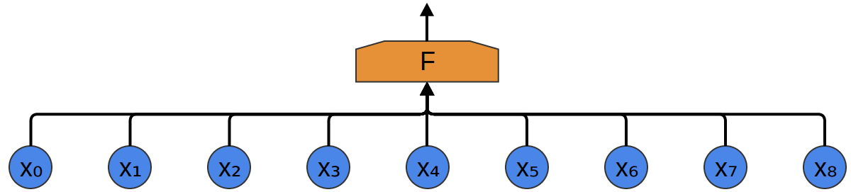
The easiest way to classify them with a neural network is to connect all samples to a fully connected layer. In addition, each input is connected to each neuron.
A more complex approach takes into account some symmetry in the properties that are in the data. We pay a lot of attention to local data properties: what is the frequency of the sound during a certain time? Increases or decreases? And so on.
We take into account the same properties at all times. It is useful to know the frequencies at the beginning, middle and at the end. Note that these are local properties, since you only need a small audio sequence window to define them.
Thus, it is possible to create a group of neurons A that consider small time segments in our data. A looks at all such segments, calculating certain functions. Then, the output of this convolutional layer is fed into a fully connected layer F.
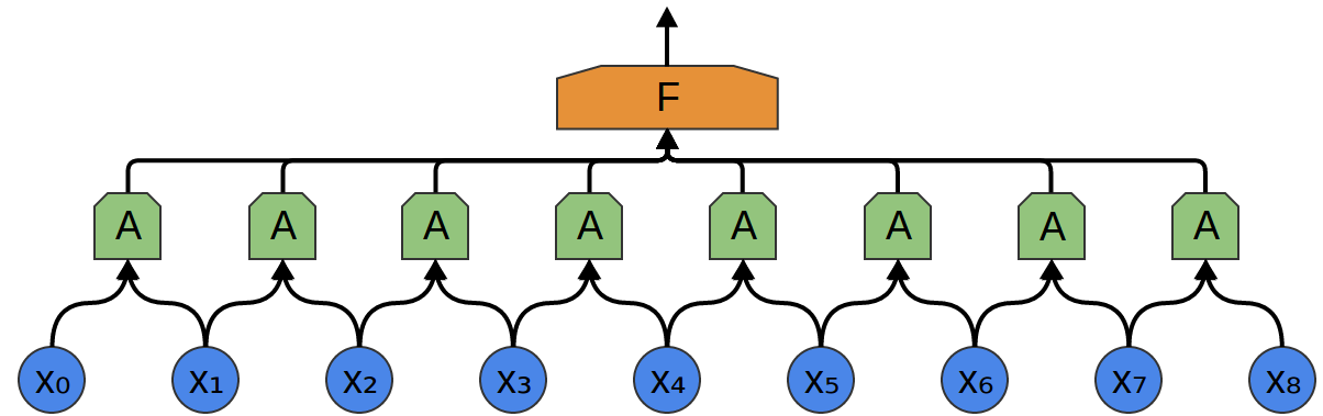
In the example above, A processed only segments consisting of two points. This is rare in practice. Normally, the convolution layer window is much larger.
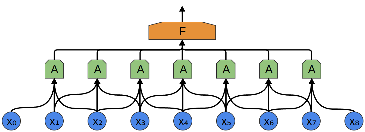
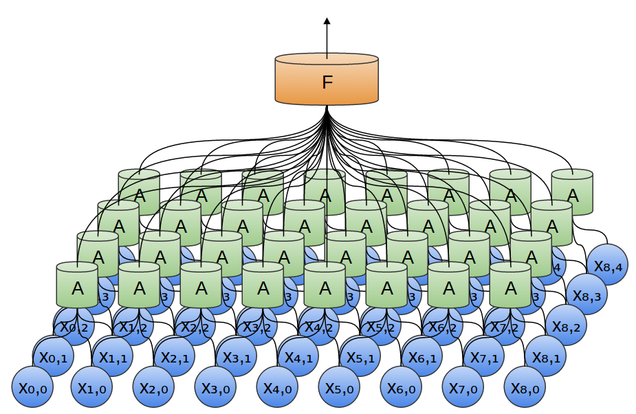
In the following example, A gets 3 slots as input. This is also unlikely for real-world tasks, but, unfortunately, it is difficult to visualize A, which connects multiple inputs.
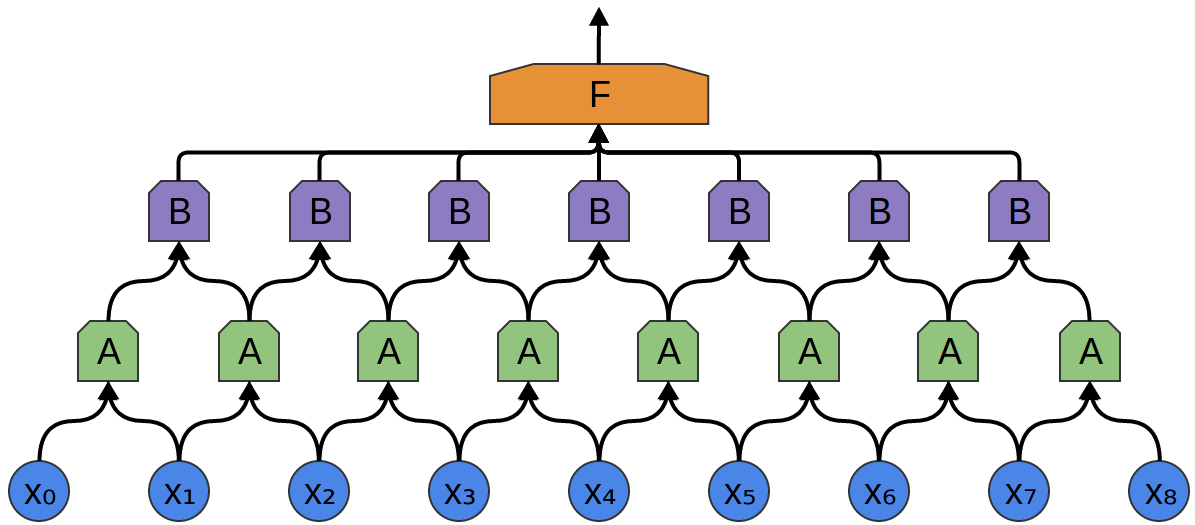
One nice feature of convolutional layers is that they are composite. You can feed one convolutional layer to another. With each layer, the network detects higher, more abstract functions.
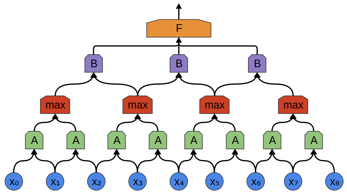
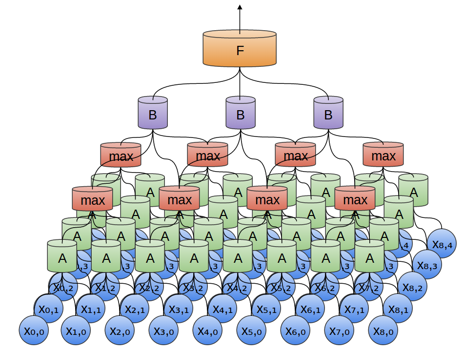
In the following example, there is a new group of neurons B. B is used to create another convolutional layer laid over the previous one.
Convolutional layers are often interwoven by pooling (unifying) layers. In particular, there is a kind of layer called max-pooling, which is extremely popular.
Often, we do not care about the exact moment in time when a useful signal is present in the data. If the signal frequency changes earlier or later, does this matter?
Max-pooling absorbs a maximum of features from small blocks of the previous level. The output says if the useful signal of the function was present in the previous layer, but not exactly where.
Max-pooling layers is “shrinking”. It allows later convolutional layers to work on large pieces of data, because small patches after the merge layer correspond to a much larger patch in front of it. They also make us invariant to some very small data transformations.
In our previous examples, one-dimensional convolutional layers were used. However, convolutional layers can work with larger data. In fact, the most well-known solutions based on convolutional neural networks use two-dimensional convolutional neural networks for pattern recognition.
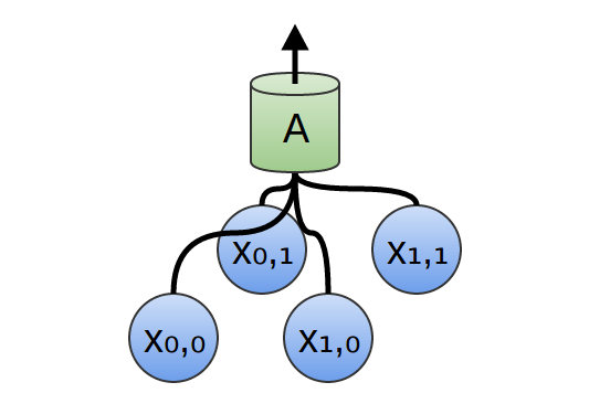
In a two-dimensional convolutional layer, instead of looking at the segments, A will look at the patches.
For each patch, A will calculate the function. For example, she can learn to detect the presence of an edge, or a texture, or a contrast between two colors.
In the previous example, the output of a convolutional layer was fed into a fully connected layer. But it is possible to compose two convolutional layers, as was the case in the one-dimensional case considered.
We can also perform max-pooling in two dimensions. Here we take a maximum of features from a small patch.
It comes down to the fact that when viewing a whole image, the exact position of the edge, up to the pixel, is not important. Enough to know where it is within a few pixels.
Also, three-dimensional convolutional networks are sometimes used for such data, such as video or volumetric data (for example, 3D scanning in medicine). However, such networks are not very widely used, and much more difficult to visualize.
Earlier, we said that A is a group of neurons. We will be more accurate in that: what is A?
In traditional convolutional layers, A is a parallel bundle of neurons; all neurons receive the same input signals and calculate different functions.
For example, in a two-dimensional convolutional layer, one neuron can detect horizontal edges, another, vertical edges, and a third green-red color contrasts.
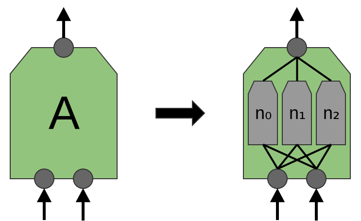
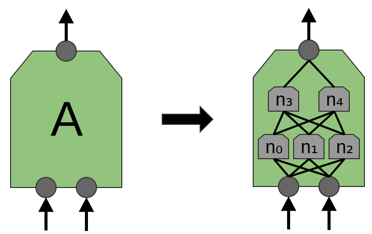
The article 'Network in Network' (Lin et al. (2013)) proposes a new layer “Mlpconv”. In this model, A has several levels of neurons, with the last layer outputting higher-level functions for the region being processed. In the article, the model achieves impressive results, establishing a new level of technology in a number of reference data sets.
For the purposes of this publication, we will focus on standard convolutional layers.
Results of convolutional neural networks
In 2012, Alex Krizhevsky, Ilya Sutskever, and Geoff Hinton achieved a significant improvement in the quality of recognition in comparison with the solutions known at that time (Krizehvsky et al. (2012)).
Progress was the result of combining several approaches. Graphic processors were used to train a large (by the standards of 2012), deep neural network. A new type of neuron (ReLU) and a new technique to reduce the problem, called “overfitting” (DropOut), were used. Used a large data set with a large number of image categories (ImageNet). And of course, it was a convolutional neural network.
The architecture shown below was deep. It has 5 convolutional layers, alternating 3 pooling and three fully connected layers.
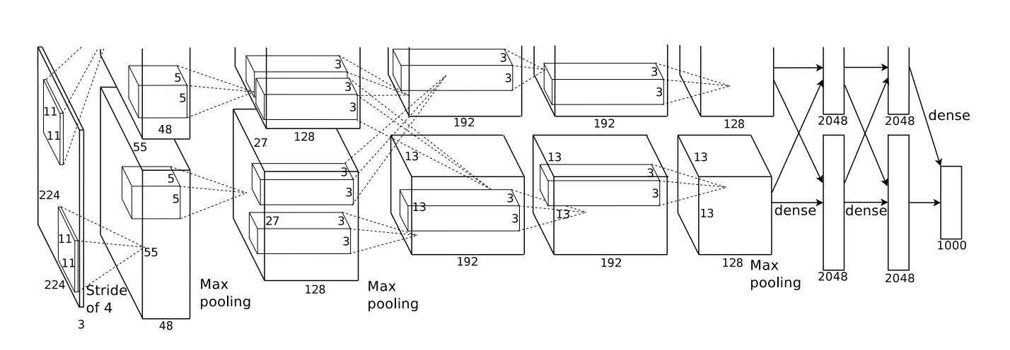
From Krizehvsky et al. (2012)
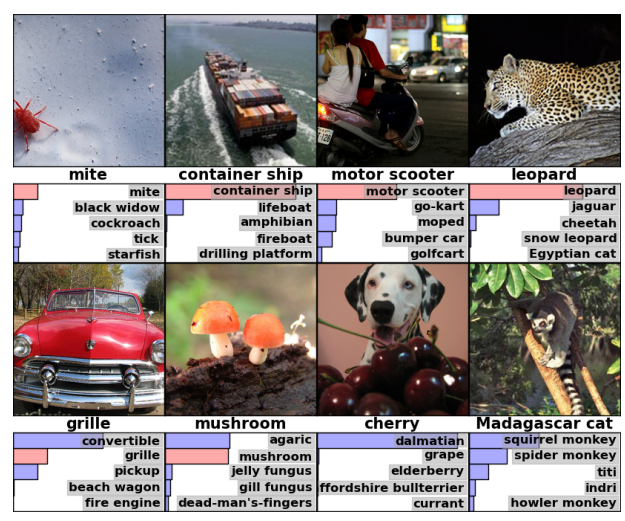
The network was trained to classify photos into thousands of different categories.
The model of Krizhevsky and others was able to give the correct answer in 63% of cases. In addition, the correct answer from the 5 best answers, there is 85% of the forecasts!
We illustrate what the first level of the network recognizes.
Recall that convolutional layers were divided between two graphics processors. Information does not go back and forth on each layer. It turns out that every time a model is launched, both sides specialize.
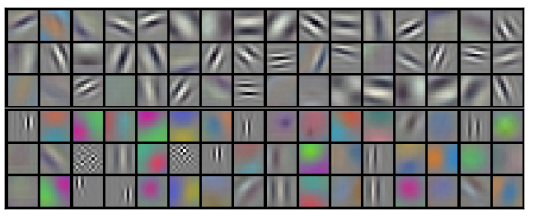
Filters obtained by the first convolutional layer. The top half corresponds to a layer on one GPU, the bottom half is on the other. From Krizehvsky et al. (2012)
Neurons from one side focus on black and white, learning to detect edges of different orientations and sizes. Neurons, on the other hand, specialize in color and texture, displaying color contrasts and patterns. Remember that neurons are randomly initialized. Not a single person went and set them up with border detectors, or divided them in this way. This happened while teaching the network to classify images.
These remarkable results (and other exciting results around that time) were just the beginning. They were quickly followed by many other papers that tested the modified approaches and gradually improved the results or applied them in other areas.
Convolutional neural networks are an important tool in computer vision and modern pattern recognition.
Consider a one-dimensional convolutional layer with inputs {xn} and outputs {yn}: It is
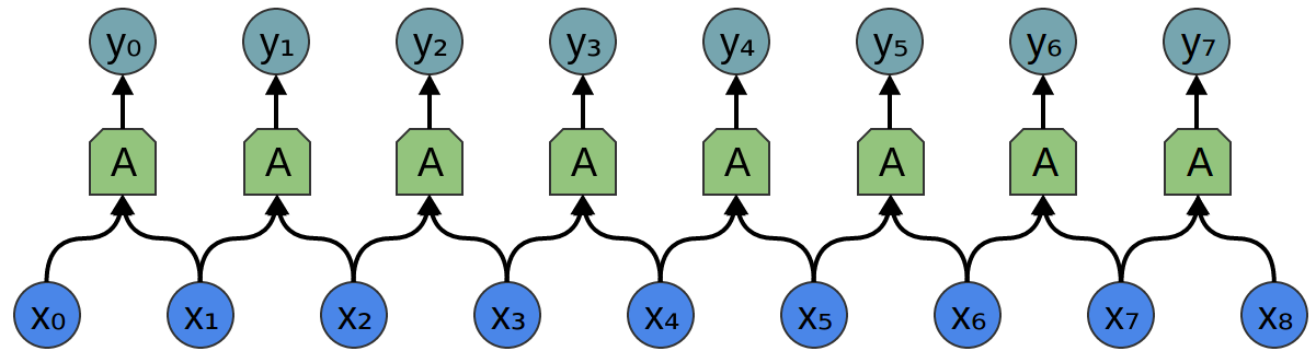
relatively easy to describe the results in terms of input data:
yn = A (x, x + 1, ...)
For example, in the example above:
y0 = A (x0 , x1)
y1 = А (x1, x2)
Similarly, if we consider a two-dimensional convolutional layer with inputs {xn, m} and conclusions {yn, m}:
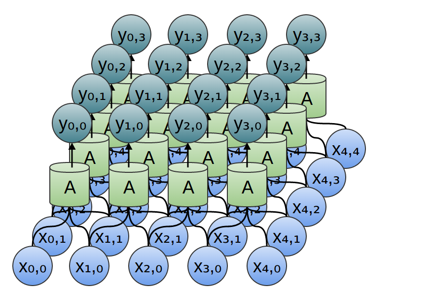
The network can be represented by a two-dimensional matrix of values.
The convolution operation is a powerful tool. In mathematics, the convolution operation occurs in different contexts, starting from the study of partial differential equations and ending with the theory of probability. Partly because of its role in the PDE, convolution is important in the physical sciences. Convolution also plays an important role in many application areas, such as computer graphics and signal processing.
Basically, a convolutional neural network can be viewed as a neural network that uses multiple identical copies of the same neuron. This allows the network to have a limited number of parameters when calculating large models.
2D convolutional neural network
This technique with multiple copies of the same neuron has a close analogy with the abstraction of functions in mathematics and computer science. When programming, the function is written once and then reused, without requiring to write the same code many times in different places, which speeds up the execution of the program and reduces the number of errors. Similarly, a convolutional neural network, once having trained a neuron, uses it in many places, which facilitates the training of the model and minimizes errors.
Structure of convolutional neural networks
Suppose a task is given in which you want to predict by audio whether there is a person’s voice in the audio file.
At the entrance we get audio samples at different points in time. Samples are evenly distributed.
The easiest way to classify them with a neural network is to connect all samples to a fully connected layer. In addition, each input is connected to each neuron.
A more complex approach takes into account some symmetry in the properties that are in the data. We pay a lot of attention to local data properties: what is the frequency of the sound during a certain time? Increases or decreases? And so on.
We take into account the same properties at all times. It is useful to know the frequencies at the beginning, middle and at the end. Note that these are local properties, since you only need a small audio sequence window to define them.
Thus, it is possible to create a group of neurons A that consider small time segments in our data. A looks at all such segments, calculating certain functions. Then, the output of this convolutional layer is fed into a fully connected layer F.
In the example above, A processed only segments consisting of two points. This is rare in practice. Normally, the convolution layer window is much larger.
In the following example, A gets 3 slots as input. This is also unlikely for real-world tasks, but, unfortunately, it is difficult to visualize A, which connects multiple inputs.
One nice feature of convolutional layers is that they are composite. You can feed one convolutional layer to another. With each layer, the network detects higher, more abstract functions.
In the following example, there is a new group of neurons B. B is used to create another convolutional layer laid over the previous one.
Convolutional layers are often interwoven by pooling (unifying) layers. In particular, there is a kind of layer called max-pooling, which is extremely popular.
Often, we do not care about the exact moment in time when a useful signal is present in the data. If the signal frequency changes earlier or later, does this matter?
Max-pooling absorbs a maximum of features from small blocks of the previous level. The output says if the useful signal of the function was present in the previous layer, but not exactly where.
Max-pooling layers is “shrinking”. It allows later convolutional layers to work on large pieces of data, because small patches after the merge layer correspond to a much larger patch in front of it. They also make us invariant to some very small data transformations.
In our previous examples, one-dimensional convolutional layers were used. However, convolutional layers can work with larger data. In fact, the most well-known solutions based on convolutional neural networks use two-dimensional convolutional neural networks for pattern recognition.
In a two-dimensional convolutional layer, instead of looking at the segments, A will look at the patches.
For each patch, A will calculate the function. For example, she can learn to detect the presence of an edge, or a texture, or a contrast between two colors.
In the previous example, the output of a convolutional layer was fed into a fully connected layer. But it is possible to compose two convolutional layers, as was the case in the one-dimensional case considered.
We can also perform max-pooling in two dimensions. Here we take a maximum of features from a small patch.
It comes down to the fact that when viewing a whole image, the exact position of the edge, up to the pixel, is not important. Enough to know where it is within a few pixels.
Also, three-dimensional convolutional networks are sometimes used for such data, such as video or volumetric data (for example, 3D scanning in medicine). However, such networks are not very widely used, and much more difficult to visualize.
Earlier, we said that A is a group of neurons. We will be more accurate in that: what is A?
In traditional convolutional layers, A is a parallel bundle of neurons; all neurons receive the same input signals and calculate different functions.
For example, in a two-dimensional convolutional layer, one neuron can detect horizontal edges, another, vertical edges, and a third green-red color contrasts.
The article 'Network in Network' (Lin et al. (2013)) proposes a new layer “Mlpconv”. In this model, A has several levels of neurons, with the last layer outputting higher-level functions for the region being processed. In the article, the model achieves impressive results, establishing a new level of technology in a number of reference data sets.
For the purposes of this publication, we will focus on standard convolutional layers.
Results of convolutional neural networks
In 2012, Alex Krizhevsky, Ilya Sutskever, and Geoff Hinton achieved a significant improvement in the quality of recognition in comparison with the solutions known at that time (Krizehvsky et al. (2012)).
Progress was the result of combining several approaches. Graphic processors were used to train a large (by the standards of 2012), deep neural network. A new type of neuron (ReLU) and a new technique to reduce the problem, called “overfitting” (DropOut), were used. Used a large data set with a large number of image categories (ImageNet). And of course, it was a convolutional neural network.
The architecture shown below was deep. It has 5 convolutional layers, alternating 3 pooling and three fully connected layers.
From Krizehvsky et al. (2012)
The network was trained to classify photos into thousands of different categories.
The model of Krizhevsky and others was able to give the correct answer in 63% of cases. In addition, the correct answer from the 5 best answers, there is 85% of the forecasts!
We illustrate what the first level of the network recognizes.
Recall that convolutional layers were divided between two graphics processors. Information does not go back and forth on each layer. It turns out that every time a model is launched, both sides specialize.
Filters obtained by the first convolutional layer. The top half corresponds to a layer on one GPU, the bottom half is on the other. From Krizehvsky et al. (2012)
Neurons from one side focus on black and white, learning to detect edges of different orientations and sizes. Neurons, on the other hand, specialize in color and texture, displaying color contrasts and patterns. Remember that neurons are randomly initialized. Not a single person went and set them up with border detectors, or divided them in this way. This happened while teaching the network to classify images.
These remarkable results (and other exciting results around that time) were just the beginning. They were quickly followed by many other papers that tested the modified approaches and gradually improved the results or applied them in other areas.
Convolutional neural networks are an important tool in computer vision and modern pattern recognition.
Formalization of convolutional neural networks
Consider a one-dimensional convolutional layer with inputs {xn} and outputs {yn}: It is
relatively easy to describe the results in terms of input data:
yn = A (x, x + 1, ...)
For example, in the example above:
y0 = A (x0 , x1)
y1 = А (x1, x2)
Similarly, if we consider a two-dimensional convolutional layer with inputs {xn, m} and conclusions {yn, m}:
The network can be represented by a two-dimensional matrix of values.
Conclusion
The convolution operation is a powerful tool. In mathematics, the convolution operation occurs in different contexts, starting from the study of partial differential equations and ending with the theory of probability. Partly because of its role in the PDE, convolution is important in the physical sciences. Convolution also plays an important role in many application areas, such as computer graphics and signal processing.