Irregular tiles on the surface of procedurally generated planets
Here we will consider a method for dividing the spherical surface of a procedurally generated planet with irregular tiles, and, as a consequence, dividing the ocean and continents into separate sections (sectors). We assume that on the surface of the planet the structure of land areas has already been set using some GIS and it is possible to export vector data to ESRI shapefiles or directly to a PostgreSQL database with the PostGIS extension . The process of creating sectors is carried out using PostGIS.
See the link to the script with SQL code at the bottom of the post, here the explanation will be more on-the-finger. The explanation provides the basic functions from the script, and also assumes the availability of data for continents and rivers of procedurally generated planets taken from forgedmaps.com .
The choice of irregular tiles allows us to accurately subdivide the surface of the planet
into sectors, never mixing the territories of the ocean and land anywhere.
We consider lakes and inland seas to be part of the land. We will also see how rivers can be used as natural boundaries of sectors. The sectors themselves will be built on the basis of some basic division of the sphere by polygons.
When it comes to dividing a flat region, they usually resort to the Voronoi diagram to obtain irregular tiles . Applying also the Lloyd algorithm, you can come to a visually attractive appearance of convex polygons that are not very different in size (Centroidal Voronoi tessellation). The essence of the Lloyd's algorithm is to repeat the construction of the Voronoi diagram, at each subsequent iteration, taking the centers of the polygons obtained at the previous iteration as generating points.
We will impose certain requirements on the basic division of spheres by polygons: the
convexity of spherical polygons and their not very large deviations from a given average size. Sector
name is used instead of tiledue to the fact that the tile usually has an elementary meaning, for example, as a unit part of the tile cards of strategic games, or as a unit part of a certain surface. Inside the sector there is an internal structure: the relief and various geographical objects in it. Sectors, in turn, can also serve as elementary tiles: building a graph of possible transitions between sectors serves this purpose.
PostGIS has a function
What happens if you try to use a straightforward approach? A rectangular projection of the planet can be converted to a square by coordinates, build polygons there and perform the inverse transformation of coordinates. But, the rectangles constructed in this way will be stretched in one direction, which would be undesirable. And, if you try to apply the Lloyd's algorithm, then the rectangles close to the poles of the sphere will be significantly smaller in area (on the sphere) than close to the equator.
Let's try to adapt this method with the elimination of disadvantages. The random starting points of the Voronoi diagram are chosen so that they are evenly distributed on the sphere. In the Mercator projection, this means that to the poles they should appear less often with a probability proportional to the cosine of latitude. We are building the Voronoi diagram in the “world” polygon - this is either the entire rectangular projection of the planet or only part of it. The function
We look at the picture of Voronoi polygons obtained in an adapted way. Here is a portion of the test planet map from the equator at the upper edge to 73 degrees south latitude at the lower edge. (Here the land area has already been cut out of landfills.)
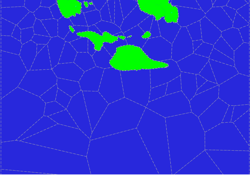
As can be seen on the Mercator projection, polygons are usually larger when approaching the poles, but they will be approximately equally distributed over the sphere in terms of area size. That's what we need. But, it is also seen that the polygons have a very large spread of areas and the overall picture is rather unsightly.
Let's try to apply several iterations of the Lloyd algorithm. As new points
for subsequent iterations of the Voronoi diagram, we will choose the centers of the
Voronoi polygons already trimmed by the “world” polygon. And to prevent too much reduction in the area of polygons near the poles, we do only a small number of iterations (3 or so).
To obtain ocean segments, the land occupied area is excluded from the obtained landfills. As a result, small polygons can be formed, which it is desirable to attach to neighboring ones. Also, small polygons may be near the border of the “world” polygon. We connect the polygons in such a way as to select the “closest” neighbor and not to spoil the big picture.
After applying such a modified algorithm, we obtain the following picture, which may already be acceptable. Red segments in the figure indicate the desired merging of the polygons.

The selection of polygons for merging can be done in different ways. In the mentioned script, 2 methods are implemented: on the longest border and on the nearest center. The following figure shows the result of the merger in the second way.
In general, we have achieved what can be desired from the ocean sectors. Their area is approximately the same (on the sphere), and they are either convex or with small deviations from the convexity.
The main function for generating ocean sectors:
Example. We are building sectors in a given “world” landfill with an average area of base landfills of 1,000,000 km 2 . Sectors whose area is smaller than half of this size will be joined to others. The second method of merging is used - at the nearest center.
On the mainland, you can enter a more interesting division, based, on the one hand, on the totality of small basic polygons, and on the other, on natural objects such as rivers and watersheds. The structure thus obtained is very similar to the map of states and provinces in them. That is, this is the process of procedurally generating the political map of the world .
Unlike ocean segments, bulge becomes completely optional.
There are no watersheds at forgedmaps.com yet, but there are already rivers. Using rivers in a script requires their representation in a MultiLineString . They have this idea in the riversz shapefile. When importing to the database, you can immediately get rid of the excess z-coordinate in this process. Other required data, namely the boundaries of land areas, are in the lands shapefile . Each land area has an identifier
For our example, we choose the average sector size of 40,000 km 2 and the average size of the base polygon of 5,000 km 2 . This is a fairly large size, chosen so for illustration only. Smaller sizes are also acceptable (up to a few m 2 ), but keep track of the calculation time and use the appropriate database configuration.
In this picture, an example of how the basic polygons look inside the land area.

The next step is to combine the base polygons into sectors. To do this, randomly select from the base polygons as many sectors as we want to make and gradually attach neighboring polygons to the accumulating sectors.
Now is the time to take river into account. We use them to divide sectors into
separate parts by function
Now we can see how some borders go along the rivers.

We connect small parts of sectors to large sectors. But we must try
Do not attach parts to the same sectors from which they were cut off.

With large areas of land we managed, but still small islands. We make those of them that have an area close to the average area of the sector as separate sectors at once. But with those whose area is much smaller than the average sector, we are doing two things.
1. If such islands are located relatively far from existing sectors, then we make them separate sectors. “Farness” here depends on the given average area of the sector: the smaller this area, the more likely it is that the island will become a separate sector.
2. If the island is close to other sectors already created, then it is combined with one of them. Namely, with the one that has the largest area in a certain polygon obtained using

Here four islands fell into two different sectors. If you increase the set average sector area, sooner or later all the islands will fall into one single sector.
The main function for generating sectors on land:
In the following example, using the function will create sectors on a plot of land with aid = 5. In this case, basic polygons with an average area of 5,000 km 2 will be used to create sectors with an average area of 40,000 km 2. Also, at the same time, the maximum territory cut off by rivers will be 0.125 * 40,000 km 2 , and 0.25 * 40,000 km 2 is the minimum area at which the islands immediately become sectors. To cut sectors by rivers, rivers with a minimum final runoff of 2 are used.
SQL script code is available that does all the work, including creating sectors and building transition graphs between neighboring sectors. GIS data from procedurally generated planets can be taken from forgedmaps.com . You can use GIS Earth data , leading them to a similar structure. You can also, using any modern GIS , make data manually from scratch or obtain new data by converting data received from any other source. More complete instructions for the script can be found in the manual .
See the link to the script with SQL code at the bottom of the post, here the explanation will be more on-the-finger. The explanation provides the basic functions from the script, and also assumes the availability of data for continents and rivers of procedurally generated planets taken from forgedmaps.com .
The choice of irregular tiles allows us to accurately subdivide the surface of the planet
into sectors, never mixing the territories of the ocean and land anywhere.
We consider lakes and inland seas to be part of the land. We will also see how rivers can be used as natural boundaries of sectors. The sectors themselves will be built on the basis of some basic division of the sphere by polygons.
When it comes to dividing a flat region, they usually resort to the Voronoi diagram to obtain irregular tiles . Applying also the Lloyd algorithm, you can come to a visually attractive appearance of convex polygons that are not very different in size (Centroidal Voronoi tessellation). The essence of the Lloyd's algorithm is to repeat the construction of the Voronoi diagram, at each subsequent iteration, taking the centers of the polygons obtained at the previous iteration as generating points.
We will impose certain requirements on the basic division of spheres by polygons: the
convexity of spherical polygons and their not very large deviations from a given average size. Sector
name is used instead of tiledue to the fact that the tile usually has an elementary meaning, for example, as a unit part of the tile cards of strategic games, or as a unit part of a certain surface. Inside the sector there is an internal structure: the relief and various geographical objects in it. Sectors, in turn, can also serve as elementary tiles: building a graph of possible transitions between sectors serves this purpose.
The basic division of the sphere and segments of the oceans.
PostGIS has a function
ST_VoronoiPolygonsthat builds a Voronoi diagram in a square area. Let's see how we can use it for our purposes. What happens if you try to use a straightforward approach? A rectangular projection of the planet can be converted to a square by coordinates, build polygons there and perform the inverse transformation of coordinates. But, the rectangles constructed in this way will be stretched in one direction, which would be undesirable. And, if you try to apply the Lloyd's algorithm, then the rectangles close to the poles of the sphere will be significantly smaller in area (on the sphere) than close to the equator.
Let's try to adapt this method with the elimination of disadvantages. The random starting points of the Voronoi diagram are chosen so that they are evenly distributed on the sphere. In the Mercator projection, this means that to the poles they should appear less often with a probability proportional to the cosine of latitude. We are building the Voronoi diagram in the “world” polygon - this is either the entire rectangular projection of the planet or only part of it. The function
ST_VoronoiPolygonsitself completes the rectangle to a square, we only need to crop the resulting diagram according to the "world" polygon. We look at the picture of Voronoi polygons obtained in an adapted way. Here is a portion of the test planet map from the equator at the upper edge to 73 degrees south latitude at the lower edge. (Here the land area has already been cut out of landfills.)
As can be seen on the Mercator projection, polygons are usually larger when approaching the poles, but they will be approximately equally distributed over the sphere in terms of area size. That's what we need. But, it is also seen that the polygons have a very large spread of areas and the overall picture is rather unsightly.
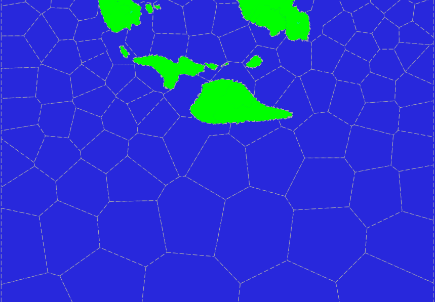
Let's try to apply several iterations of the Lloyd algorithm. As new points
for subsequent iterations of the Voronoi diagram, we will choose the centers of the
Voronoi polygons already trimmed by the “world” polygon. And to prevent too much reduction in the area of polygons near the poles, we do only a small number of iterations (3 or so).
To obtain ocean segments, the land occupied area is excluded from the obtained landfills. As a result, small polygons can be formed, which it is desirable to attach to neighboring ones. Also, small polygons may be near the border of the “world” polygon. We connect the polygons in such a way as to select the “closest” neighbor and not to spoil the big picture.
After applying such a modified algorithm, we obtain the following picture, which may already be acceptable. Red segments in the figure indicate the desired merging of the polygons.
The selection of polygons for merging can be done in different ways. In the mentioned script, 2 methods are implemented: on the longest border and on the nearest center. The following figure shows the result of the merger in the second way.
In general, we have achieved what can be desired from the ocean sectors. Their area is approximately the same (on the sphere), and they are either convex or with small deviations from the convexity.
The main function for generating ocean sectors:
map.makeOceanSectors(
    world Geometry,
    avg_vp_areaKM Double Precision,
    merging_ratio Double Precision,
    merging_method Int
    ) RETURNS Void
world- A “world” training ground serving as the borders of the world. avg_vp_areaKM- the average area (km 2 ) of polygons from which the ocean sectors are made. merging_ratio- share avg_vp_areaKM, such that if the sector area is less than it, then it will be attached to the neighboring one. merging_method- merge method ('1' or '2'). Example. We are building sectors in a given “world” landfill with an average area of base landfills of 1,000,000 km 2 . Sectors whose area is smaller than half of this size will be joined to others. The second method of merging is used - at the nearest center.
SELECT * FROM map.makeOceanSectors( ST_GeomFromText(
    'POLYGON((-75 -85, 75 -85, 75 85, -75 85, -75 -85))', 4326 ),
    1000000, 0.5, 2
);
Segments of the continents.
On the mainland, you can enter a more interesting division, based, on the one hand, on the totality of small basic polygons, and on the other, on natural objects such as rivers and watersheds. The structure thus obtained is very similar to the map of states and provinces in them. That is, this is the process of procedurally generating the political map of the world .
Unlike ocean segments, bulge becomes completely optional.
There are no watersheds at forgedmaps.com yet, but there are already rivers. Using rivers in a script requires their representation in a MultiLineString . They have this idea in the riversz shapefile. When importing to the database, you can immediately get rid of the excess z-coordinate in this process. Other required data, namely the boundaries of land areas, are in the lands shapefile . Each land area has an identifier
aid(area Id) and may consist of the continent and the nearest islands, or only of small islands located nearby. For our example, we choose the average sector size of 40,000 km 2 and the average size of the base polygon of 5,000 km 2 . This is a fairly large size, chosen so for illustration only. Smaller sizes are also acceptable (up to a few m 2 ), but keep track of the calculation time and use the appropriate database configuration.
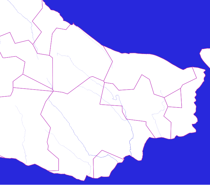
In this picture, an example of how the basic polygons look inside the land area.
The next step is to combine the base polygons into sectors. To do this, randomly select from the base polygons as many sectors as we want to make and gradually attach neighboring polygons to the accumulating sectors.
Now is the time to take river into account. We use them to divide sectors into
separate parts by function
ST_Split. Such a division can be performed depending on some conditions: the final river flow or the area of the separated part. Now we can see how some borders go along the rivers.
We connect small parts of sectors to large sectors. But we must try
Do not attach parts to the same sectors from which they were cut off.
With large areas of land we managed, but still small islands. We make those of them that have an area close to the average area of the sector as separate sectors at once. But with those whose area is much smaller than the average sector, we are doing two things.
1. If such islands are located relatively far from existing sectors, then we make them separate sectors. “Farness” here depends on the given average area of the sector: the smaller this area, the more likely it is that the island will become a separate sector.
2. If the island is close to other sectors already created, then it is combined with one of them. Namely, with the one that has the largest area in a certain polygon obtained using
ST_Bufferfrom this island. Here four islands fell into two different sectors. If you increase the set average sector area, sooner or later all the islands will fall into one single sector.
The main function for generating sectors on land:
map.makeLandSectors(
    aid BigInt,
    avg_vp_areaKM Double Precision,
    avg_sector_areaKM Double Precision,
    max_sector_cut_area_ratio Float,
    pref_min_island_area_ratio Float,
    min_streamflow Int
    ) RETURNS Void
aid- identifier of the land area. avg_vp_areaKM- the average area (km 2 ) of the base landfills. avg_sector_areaKM- average area (km 2 ) of sectors. max_sector_cut_area_ratio- the fraction avg_sector_areaKMthat defines the maximum area that can be cut off by the river. pref_min_island_area_ratio- the share avg_sector_areaKMthat determines the minimum area, having which the island immediately becomes a separate sector. streamflow- if the river has a final runoff not less than this value, then it participates in cutting sectors. In the following example, using the function will create sectors on a plot of land with aid = 5. In this case, basic polygons with an average area of 5,000 km 2 will be used to create sectors with an average area of 40,000 km 2. Also, at the same time, the maximum territory cut off by rivers will be 0.125 * 40,000 km 2 , and 0.25 * 40,000 km 2 is the minimum area at which the islands immediately become sectors. To cut sectors by rivers, rivers with a minimum final runoff of 2 are used.
SELECT * FROM map.makeLandSectors(5, 5000, 40000, 0.125, 0.25, 2);
References
SQL script code is available that does all the work, including creating sectors and building transition graphs between neighboring sectors. GIS data from procedurally generated planets can be taken from forgedmaps.com . You can use GIS Earth data , leading them to a similar structure. You can also, using any modern GIS , make data manually from scratch or obtain new data by converting data received from any other source. More complete instructions for the script can be found in the manual .