The basics of fractal image compression
Fractals are amazing mathematical objects that captivate with their simplicity and rich capabilities for constructing objects of complex nature with just a few coefficients and a simple iterative scheme.
It is these capabilities that make it possible to use them for image compression, especially for nature photographs and other complex self-similar images.
In this article I will try to briefly answer the simple question: "How is this done?"
To begin with, you still have to go a little deeper into mathematics and introduce several definitions.
The following will come in handy:
Compression mappings have an important property. If we take any point and start iteratively applying the same contraction map to it: f (f (f (f ... f (x))), then the result will always be the same point. The more times we apply, the more accurately we find this point. It is called a fixed point, and for each compressive mapping it exists, and only one.
Several affine compressive mappings form a system of iterated functions (CIF). In fact, CIF is a multiplier machine. It takes the original image, distorts it, moves it, and so on several times.
For example, this is how, using CIF, of three functions, a Sierpinski triangle is built:
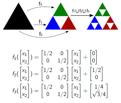
The original triangle multiplies three times, decreases and is transferred. Etc. If we continue this way to infinity, we get a well-known fractal with an area of 0 and a dimension of 1.585.
If the functions included in the CIF are compressive, then the CIF itself also has a fixed point. But this “point” will no longer be a familiar point in N-dimensional space, but a set of such points, that is, an image. It is called a CIF attractor . For the CIF, above, the Sierpinski triangle will be an attractor.
Here we go to the next level - the image space. In this space:
Having a CIF, finding an attractor is easy. In any case, having a computer at hand. You can take absolutely any initial image and start applying CIF to it. An example with the same triangle, but already built from a square:

It turns out that to construct a rather complex figure, we needed 18 coefficients. The gain, as they say, is obvious.
Now, if we knew how to solve the inverse problem - having an attractor, building a CIF ... Then it’s enough to take an attractor image similar to your cat’s photo and you can code it pretty profitably.
Here, in fact, the problems begin. Arbitrary images, unlike fractals, are not self-similar, so this task is not so easily solved. How to do this was invented in 1992 by Arnold Jacquin, while he was graduate student Michael Barnsley, who is considered the father of fractal compression.
We need self-similarity - otherwise affine transformations, limited in their capabilities, will not be able to bring images closer to reality. And if it is not between the part and the whole, then you can search between the part and the part. Apparently, Jacquin reasoned roughly the same way.
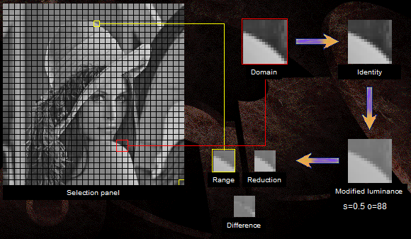
A simplified coding scheme looks like this:
In the picture, the ranking block is marked in yellow, the corresponding domain one is in red. Transformation steps and result are also shown.
You can play it yourself: Coder demo .
Obtaining the optimal transformation is a separate issue, but it is not a big deal. But another drawback of the circuit is visible to the naked eye. You can calculate how many 32 × 32 domain blocks a two-megapixel image contains. Their exhaustive search for each rank block is the main problem of this type of compression - coding takes a very long time. Of course, they are struggling with this using various tricks, such as narrowing the search area or preliminary classification of domain blocks. With various damage to quality.
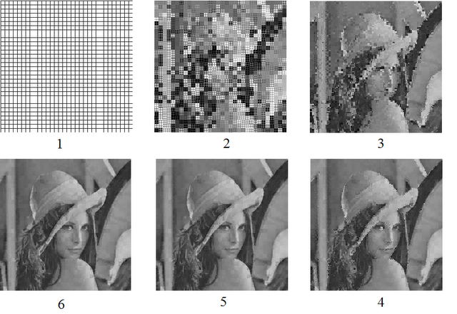
Decoding is simple and fairly quick. We take any image, divide it into ranking areas, successively replace them with the result of applying resp. conversion to acc. domain area (whatever it contains at the moment). After several iterations, the original image will look like itself:
Perhaps, for the introduction of information is enough. Those interested can read the relevant articles on Wikipedia or the relevant community .
A detailed exposition can be found in this article , with which it all began in 1992. Most of the materials, of course, are in English.
It is these capabilities that make it possible to use them for image compression, especially for nature photographs and other complex self-similar images.
In this article I will try to briefly answer the simple question: "How is this done?"
To begin with, you still have to go a little deeper into mathematics and introduce several definitions.
The following will come in handy:
- A metric is a function defined on a space that returns the distance between two points of this space. For example, the usual Euclidean metric. If a space metric is given, it is called metric. The metric should satisfy certain conditions, but we will not go deep.
- A contraction mapping (transformation) is a function on metric space that uniformly reduces the distance between two points in space. For example, y = 0.5x.
Compression mappings have an important property. If we take any point and start iteratively applying the same contraction map to it: f (f (f (f ... f (x))), then the result will always be the same point. The more times we apply, the more accurately we find this point. It is called a fixed point, and for each compressive mapping it exists, and only one.
Several affine compressive mappings form a system of iterated functions (CIF). In fact, CIF is a multiplier machine. It takes the original image, distorts it, moves it, and so on several times.
For example, this is how, using CIF, of three functions, a Sierpinski triangle is built:
The original triangle multiplies three times, decreases and is transferred. Etc. If we continue this way to infinity, we get a well-known fractal with an area of 0 and a dimension of 1.585.
If the functions included in the CIF are compressive, then the CIF itself also has a fixed point. But this “point” will no longer be a familiar point in N-dimensional space, but a set of such points, that is, an image. It is called a CIF attractor . For the CIF, above, the Sierpinski triangle will be an attractor.
Here we go to the next level - the image space. In this space:
- A point of space is an image.
- The distance between the points shows how similar the images are to each other, how “close” (naturally, if you set it accordingly).
- Compression mapping makes any two images more similar (in the sense of a given metric).
Having a CIF, finding an attractor is easy. In any case, having a computer at hand. You can take absolutely any initial image and start applying CIF to it. An example with the same triangle, but already built from a square:
It turns out that to construct a rather complex figure, we needed 18 coefficients. The gain, as they say, is obvious.
Now, if we knew how to solve the inverse problem - having an attractor, building a CIF ... Then it’s enough to take an attractor image similar to your cat’s photo and you can code it pretty profitably.
Here, in fact, the problems begin. Arbitrary images, unlike fractals, are not self-similar, so this task is not so easily solved. How to do this was invented in 1992 by Arnold Jacquin, while he was graduate student Michael Barnsley, who is considered the father of fractal compression.
We need self-similarity - otherwise affine transformations, limited in their capabilities, will not be able to bring images closer to reality. And if it is not between the part and the whole, then you can search between the part and the part. Apparently, Jacquin reasoned roughly the same way.
A simplified coding scheme looks like this:
- The image is divided into small, non-overlapping square areas called rank blocks. In fact, it is divided into squares. See the picture below.
- A pool of all possible overlapping blocks of four times large ranking - domain blocks is being built.
- For each rank block, we “try on” domain blocks in turn and look for a transformation that makes the domain block most similar to the current rank one.
- The conversion-domain block pair, which has come close to the ideal, is mapped to the rank block. Conversion coefficients and coordinates of the domain block are stored in the encoded image. We don’t need the contents of the domain block - you remember, we don’t care where to start.
In the picture, the ranking block is marked in yellow, the corresponding domain one is in red. Transformation steps and result are also shown.
You can play it yourself: Coder demo .
Obtaining the optimal transformation is a separate issue, but it is not a big deal. But another drawback of the circuit is visible to the naked eye. You can calculate how many 32 × 32 domain blocks a two-megapixel image contains. Their exhaustive search for each rank block is the main problem of this type of compression - coding takes a very long time. Of course, they are struggling with this using various tricks, such as narrowing the search area or preliminary classification of domain blocks. With various damage to quality.
Decoding is simple and fairly quick. We take any image, divide it into ranking areas, successively replace them with the result of applying resp. conversion to acc. domain area (whatever it contains at the moment). After several iterations, the original image will look like itself:
Perhaps, for the introduction of information is enough. Those interested can read the relevant articles on Wikipedia or the relevant community .
A detailed exposition can be found in this article , with which it all began in 1992. Most of the materials, of course, are in English.