Tracing the path to the GPU in Unity - part 2

"There is nothing worse than a clear image of a blurred concept." - Photographer Ansel Adams

In the first part of the article, we created a Whitted ray tracer that can trace perfect reflections and sharp shadows. But we lack the effects of fuzziness: diffuse interplay, glossy reflections and soft shadows.

Based on the code we already have , we iteratively solve the rendering equation formulated by James Cajia in 1986 and transform our renderer into a path scanner capable of transmitting the above-mentioned effects. We will again use C # for scripts and HLSL for shaders. The code is laid out on Bitbucket .

This article is much more mathematical than the previous one, but do not be alarmed. I will try to explain each formula as clearly as possible. Formulas are needed here to see what is happening and why our renderer works, so I recommend trying to understand them, and if something proves incomprehensible, ask questions in the comments to the original article.

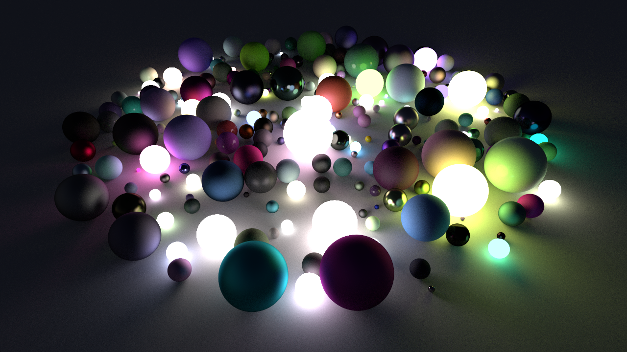
The image below is rendered using the Graffiti Shelter card from the HDRI Haven site. Other images in this article are rendered using the Kiara 9 Dusk card .

Rendering equation

From a formal point of view, the task of the photorealistic renderer is to solve the rendering equation, which is written as follows:

$$

Let's analyze it. Our ultimate goal is to determine the brightness of a pixel of the screen. The rendering equation gives us the amount of light$$outgoing from point $$ (point of incidence) towards $$(direction in which the beam falls). The surface itself can be a source of light emitting light.$$in our direction. Most surfaces do not, so they only reflect light falling outside. That is why the integral is used. It accumulates light coming from every possible direction of the hemisphere.$$around the normal (so for now we take into account the light falling on the surface from above , and not from the inside , which may be necessary for translucent materials).

First part -$$called the two-dimensional distribution function of the reflectivity of objects (bidirectional reflectance distribution function, BRDF). This function visually describes the type of material we are dealing with: metal or dielectric, dark or bright, shiny or dull. BRDF determines the proportion of lighting coming from$$which is reflected in the direction $$. In practice, this is implemented using a three-component vector with values ​​of red, green and blue in the interval$$.

The second part of -$$- this is equivalent to ¹$$where $$ - the angle between the incident light and the surface normal $$. Imagine a column of parallel rays of light falling perpendicular to the surface. Now imagine the same beam falling on a surface at a flat angle. Light will be distributed over a larger area, but it also means that every point of this area will look darker. Cosine is needed to take this into account.

Finally, the very light received from$$is defined recursively using the same equation. That is the lighting at the point$$depends on the incident light from all possible directions in the upper hemisphere. In each of these directions from the point$$ there is another point $$whose brightness again depends on the light falling from all possible directions of the upper hemisphere of this point. All calculations are repeated.

This is what happens here, this is an infinitely recursive integral equation with an infinite number of hemispherical integration domains. We will not be able to solve this equation directly, but there is a fairly simple solution.

---

¹ Do not forget about it! We will often talk about cosine, and at the same time we will always mean scalar product. Because$$, and we are dealing with directions (unit vectors), the scalar product is the cosine of most computer graphics tasks.

Monte Carlo comes to the rescue

Monte Carlo integration is a numerical integration technique that allows us to approximately calculate any integral using a finite number of random samples. Moreover, Monte Carlo guarantees convergence to the right decision - the more samples we take, the better. Here is its generalized form:

$$

Therefore, the integral of the function $$can be approximately calculated by averaging random samples in the integration domain. Each sample is divided by the probability of its choice.$$. Due to this, more often the selected sample will have more weight than the selected less often.

In the case of uniform samples on a hemisphere (each direction has the same probability of being selected), the probability of samples is constant:$$ (because $$Is the surface area of ​​a single hemisphere). If we put all this together, we get the following:

$$

Radiation $$- this is just the value returned by our function Shade.$$already performed in our function AddShader. Multiplication by$$happens when we reflect the beam and trace it further. Our task is to give life to the green part of the equation.

Prerequisites

Before we go on a journey, let's take care of some aspects: the accumulation of samples, deterministic scenes and randomness of the shader.

Accumulation

For some reason, Unity does not pass me an HDR texture as destinationin OnRenderImage. I worked the format R8G8B8A8_Typeless, so the accuracy quickly becomes too low for the accumulation of a large number of samples. To deal with this, let's add to the C # script private RenderTexture _converged. This will be our buffer, accumulating results with high accuracy before displaying them on the screen. We initialize / free the texture in the same way as _targetin the function InitRenderTexture. In function, we Renderdouble the blit:

Graphics.Blit(_target, _converged, _addMaterial);
Graphics.Blit(_converged, destination);

Deterministic scenes

When making changes to rendering to evaluate the effect, a comparison with previous results is useful. So far, each time we restart Play mode or recompilate the script, we will get a new random scene. To avoid this, add the public int SphereSeedfollowing line to the beginning of the script in C # SetUpScene:

Random.InitState(SphereSeed);

Now we can manually set the seed scene. Enter any number and disable / re-enable the component RayTracingMasteruntil you get the right scene.

For example images, the following parameters were used: Sphere Seed 1223832719, Sphere Radius [5, 30], Spheres Max 10000, Sphere Placement Radius 100.

Shader randomness

Before proceeding to stochastic sampling, we need to add randomness to the shader. I will use the canonical string I found on the network , modified for more convenience:

float2 _Pixel;
float _Seed;
floatrand()
{
    float result = frac(sin(_Seed / 100.0f * dot(_Pixel, float2(12.9898f, 78.233f))) * 43758.5453f);
    _Seed += 1.0f;
    return result;
}

We initialize _Pixeldirectly into CSMainhow _Pixel = id.xy, so that each pixel can use different random values. _Seedinitialized from C # to a function SetShaderParameters.

RayTracingShader.SetFloat("_Seed", Random.value);

The quality of random numbers generated here is unstable. In the future, it would be worth exploring and testing this function, analyzing the effect of parameters and comparing it with other approaches. But for now, we'll just use it and hope for the best.

Hemisphere Sampling

Let's start first: we need random directions evenly distributed over the hemisphere. This nontrivial task for the full sphere is described in detail in this article by Corey Simon. It is easy to adapt to the hemisphere. This is what the shader code looks like:

float3 SampleHemisphere(float3 normal)
{
    // Однородная выборка направлений полусферыfloat cosTheta = rand();
    float sinTheta = sqrt(max(0.0f, 1.0f - cosTheta * cosTheta));
    float phi = 2 * PI * rand();
    float3 tangentSpaceDir = float3(cos(phi) * sinTheta, sin(phi) * sinTheta, cosTheta);
    // Преобразование направления в пространство мираreturn mul(tangentSpaceDir, GetTangentSpace(normal));
}

Directions are generated for a hemisphere centered about the positive Z axis, so we need to transform them so that they are centered relative to the desired normal. We generate a tangent and a binormal (two vectors, orthogonal to the normal and orthogonal to each other). First we select an auxiliary vector to generate a tangent. To do this, we take the positive X axis, and return to the positive Z only if it is normal (approximately) aligned with the X axis. Then we can use the vector product to generate a tangent, and then binormal.

float3x3 GetTangentSpace(float3 normal)
{
    // Выбираем вспомогательный вектор для векторного произведения
    float3 helper = float3(1, 0, 0);
    if (abs(normal.x) > 0.99f)
        helper = float3(0, 0, 1);
    // Генерируем векторы
    float3 tangent = normalize(cross(normal, helper));
    float3 binormal = normalize(cross(normal, tangent));
    return float3x3(tangent, binormal, normal);
}

Lambert scattering

Now that we have homogeneous random directions, we can start implementing the first BRDF. For diffuse reflection, BRDF is most commonly used according to Lambert, which is surprisingly simple:$$where $$- this is albedo surface. Let's insert it into our Monte Carlo rendering equation (I’ll not take radiance into account yet) and see what happens:

$$

Let's immediately insert this equation into the shader. In the function, Shadewe replace the code inside the construction with the if (hit.distance < 1.#INF)following lines:

// Рассеянное затенение
ray.origin = hit.position + hit.normal * 0.001f;
ray.direction = SampleHemisphere(hit.normal);
ray.energy *= 2 * hit.albedo * sdot(hit.normal, ray.direction);
return0.0f;

The new direction of the reflected beam is determined using our homogeneous sample function over the hemisphere. The beam energy is multiplied by the corresponding part of the equation shown above. Since the surface does not emit any light (it only reflects light received directly or indirectly from the sky), we return 0. Here, do not forget that it AddShaderaverages the samples, so we don’t need to worry about$$. The function CSMainalready contains multiplication by$$(the next reflected beam), so there is not much work left for us.

sdotThis is a helper function that I defined for myself. It simply returns the result of the scalar product with an additional coefficient, and then limits it to$$:

floatsdot(float3 x, float3 y, float f = 1.0f)
{
    return saturate(dot(x, y) * f);
}

Let's summarize what our code is doing for now. CSMaingenerates the camera's primary rays and triggers Shade. When intersecting with the surface, this function in turn generates a new beam (uniformly random in the hemisphere around the normal) and takes into account the BRDF of the material and the cosine of the beam energy. When intersecting the ray with the sky, we sample the HDRI (our only light source) and return the light that is multiplied by the beam energy (i.e. the result of all previous intersections, starting with the camera). This is a simple sample that is mixed with a converging result. As a result, each sample takes into account the impact$$.

It is time to check everything in work. Since metals have no diffuse reflection, let's turn them off in SetUpScenethe C # script function (but still calling here Random.valueto keep the scene deterministic):

bool metal = Random.value < 0.0f;

Start the Play mode and see how the noisy image is initially cleared and converges to a beautiful rendering:

Phong mirror image

Not bad for just a few lines of code (and a small fraction of mathematics). Let's enhance the picture by adding mirror reflections using BRDF on Phong. Phong's original wording had its own problems (lack of interaction and energy conservation), but fortunately other people eliminated them . The enhanced BRDF is shown below.$$ - This is the direction of the perfectly reflected light, and $$ - this is Phong's index, managing roughness (roughness):

$$

An interactive two-dimensional graph shows what a BRDF Phong looks like when$$for a beam falling at an angle of 45 °. Try changing the value$$.

Insert this into our Monte Carlo equation:

$$

Finally, add it up with the already existing BRDF according to Lambert:

$$

And this is how they look in the code, along with Lambert scattering:

// Затенение по Фонгу
ray.origin = hit.position + hit.normal * 0.001f;
float3 reflected = reflect(ray.direction, hit.normal);
ray.direction = SampleHemisphere(hit.normal);
float3 diffuse = 2 * min(1.0f - hit.specular, hit.albedo);
float alpha = 15.0f;
float3 specular = hit.specular * (alpha + 2) * pow(sdot(ray.direction, reflected), alpha);
ray.energy *= (diffuse + specular) * sdot(hit.normal, ray.direction);
return0.0f;

Notice that we replaced the scalar product with a slightly different, but equivalent (reflected $$ instead $$). Now we will turn on the metallic materials in the functions SetUpSceneand check how it works.

Experimenting with different values$$, you can notice the problem: even low rates require a lot of time for convergence, and at high rates noise is especially striking. Even after a few minutes of waiting, the result is far from perfect, which is unacceptable for such a simple scene.$$ and $$ with 8192 samples look like this:



Why did this happen? After all, before we had such beautiful perfect reflections ($$)! .. The problem is that we generate homogeneous samples and give them weights according to BRDF. With high Phong scores, the BRDF value is small for everyone, but these directions are very close to the ideal reflection, and it is very unlikely that we will randomly select them using our homogeneous samples. On the other hand, if we actually intersect one of these directions, then BRDF will be huge to offset all the other small samples. The result is a very large dispersion. Paths with multiple specular reflections are even worse, and lead to noise that appears in the images.

Improved Sampling

To make our path tracer applicable in practice, we need to change the paradigm. Instead of spending precious samples on areas in which they end up being unimportant (since they get a very low BRDF and / or cosine value), let's generate important samples .

As a first step, we will return our ideal reflections, and then we will see how we can generalize this idea. To do this, we divide the shading logic into diffuse and specular reflection. For each sample, we will randomly choose one or the other (depending on the ratio$$ and $$). In the case of diffuse reflection, we will stick to homogeneous samples, but for a specular one, we will explicitly reflect the beam in a single important direction. Since fewer samples will now be spent on each type of reflection, we need to increase the impact accordingly in order to get the same total value:

// Вычисляем вероятности рассеянного и зеркального отражений
hit.albedo = min(1.0f - hit.specular, hit.albedo);
float specChance = energy(hit.specular);
float diffChance = energy(hit.albedo);
float sum = specChance + diffChance;
specChance /= sum;
diffChance /= sum;
// Рулеткой выбираем путь лучаfloat roulette = rand();
if (roulette < specChance)
{
    // Зеркальное отражение
    ray.origin = hit.position + hit.normal * 0.001f;
    ray.direction = reflect(ray.direction, hit.normal);
    ray.energy *= (1.0f / specChance) * hit.specular * sdot(hit.normal, ray.direction);
}
else
{
    // Рассеянное отражение
    ray.origin = hit.position + hit.normal * 0.001f;
    ray.direction = SampleHemisphere(hit.normal);
    ray.energy *= (1.0f / diffChance) * 2 * hit.albedo * sdot(hit.normal, ray.direction);
}
return0.0f;

energy is a small auxiliary function averaging color channels:

floatenergy(float3 color)
{
    return dot(color, 1.0f / 3.0f);
}

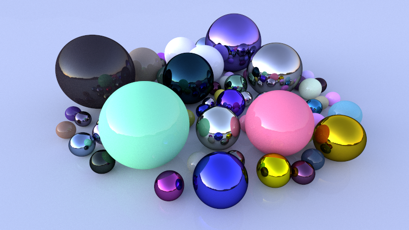
So we created a more beautiful Whitted ray tracer from the previous part, but now with real diffuse shading (which implies soft shadows, ambient occlusion, diffused global illumination):

Sampling by importance

Let's take another look at the basic Monte Carlo formula:

$$

As you can see, we divide the influence of each sample (sample) on the probability of choosing this particular sample. While we used homogeneous samples by hemisphere, we therefore had constant$$. As we saw above, this is far from optimal, for example, in the case of the Phong BRDF, which is large in a very small number of directions.

Imagine that we could find a probability distribution exactly corresponding to an integrable function:$$. Then the following will happen:

$$

Now we have no samples making a very small contribution. These samples will be selected with less probability. This will significantly reduce the variance of the result and accelerate the convergence of rendering.

In practice, it is impossible to find such an ideal distribution, because some parts of the integrable function (in our case BRDF × cosine × incident light) are unknown (this is most obvious for incident light), but the distribution of samples according to BRDF × to cosine or even just according to BRDF will greatly help us. This principle is called sampling by importance.

Sample of cosines

In the subsequent stages, we need to replace our uniform distribution of samples with the distribution according to the cosine rule. Do not forget, instead of multiplying homogeneous samples by cosine, reducing their influence, we want to generate a proportionally smaller number of samples.

In this article, Thomas Poole describes how this is done. We will add a SampleHemisphereparameter to our function alpha. The function determines the cosine sample rate: 0 for a uniform sample, 1 for a cosine sample, or higher for higher Phong values. In code, it looks like this:

float3 SampleHemisphere(float3 normal, float alpha)
{
    // Сэмплируем полусферу, где альфа определяет тип сэмплированияfloat cosTheta = pow(rand(), 1.0f / (alpha + 1.0f));
    float sinTheta = sqrt(1.0f - cosTheta * cosTheta);
    float phi = 2 * PI * rand();
    float3 tangentSpaceDir = float3(cos(phi) * sinTheta, sin(phi) * sinTheta, cosTheta);
    // Преобразуем направление в пространство мираreturn mul(tangentSpaceDir, GetTangentSpace(normal));
}

Now the probability of each sample is equal to $$. The beauty of this equation may not immediately seem obvious, but a little later you will understand it.

Lambert sampling by importance

To begin with, we will enhance the rendering of diffuse reflection. In our uniform distribution, we use the constant BRDF in Lambert, but we can improve it by adding cosine. The distribution of sampling probabilities over a cosine (where$$) equals $$That simplifies our Monte Carlo formula for diffuse reflection:

$$

// Рассеянное отражение
ray.origin = hit.position + hit.normal * 0.001f;
ray.direction = SampleHemisphere(hit.normal, 1.0f);
ray.energy *= (1.0f / diffChance) * hit.albedo;

This will speed up our diffuse shading a bit. Now let's deal with a real problem.

Phong selection by importance

For the BRDF Phong procedure is similar. This time we have the product of two cosines: the standard cosine from the rendering equation (as is the case with diffuse reflection) multiplied by the own cosmic BRDF. We will deal only with the latter.

Let's insert the probability distribution from the examples above into the Phong equation. A detailed conclusion can be explored in the article Lafortune and Willems: Using the Modified Phong Reflectance Model for Physically Based Rendering (1994) :

$$

// Зеркальное отражениеfloat alpha = 15.0f;
ray.origin = hit.position + hit.normal * 0.001f;
ray.direction = SampleHemisphere(reflect(ray.direction, hit.normal), alpha);
float f = (alpha + 2) / (alpha + 1);
ray.energy *= (1.0f / specChance) * hit.specular * sdot(hit.normal, ray.direction, f);

These changes are enough to fix any problems with high Phong scores and make our rendering converge in a much more reasonable time.

Materials

Finally, let's expand our scene generation to create varying values ​​for the smoothness and radiance of the spheres! In struct Spherefrom the script in C # add public float smoothnessand public Vector3 emission. Since we changed the size of the struct, we need to change the step when creating the Compute Buffer (4 × number of float numbers, remember?). Let the function SetUpSceneinsert the values ​​for smoothness and emissivity.

In the shader, add both variables to struct Sphereand struct RayHit, and then initialize them to CreateRayHit. And finally, set both values ​​in IntersectGroundPlane(hardcoded in the code, insert any values) and IntersectSphere(get values ​​from Sphere).

I want to use the smoothness values ​​in the same way as in the standard Unity shader, which differs from the rather arbitrary Phong index. Here is a well-functioning conversion that can be used in a function Shade:

floatSmoothnessToPhongAlpha(float s)
{
    return pow(1000.0f, s * s);
}

float alpha = SmoothnessToPhongAlpha(hit.smoothness);

The use of emissivity is performed by returning the value to Shade:

return hit.emission;

results

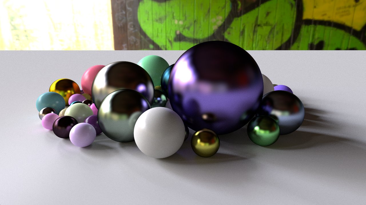
Take a deep breath. relax and wait until the image turns into such a beautiful picture:


Congratulations! You managed to get through the thicket of mathematical expressions. We implemented a path tracer that performs diffused and specular shading, learned about the sample by importance, immediately applying this concept to render the convergence in minutes, not hours or days.

Compared with the previous one, this article was a huge step in terms of complexity, but also significantly improved the quality of the result. Working with mathematical calculations takes time, but it justifies itself, because it can significantly deepen your understanding of what is happening and allow you to expand the algorithm without destroying physical certainty.

Thanks for reading! In the third part, we (for a while) will emerge from the jungle of sampling and shading, and return to civilization to meet with gentlemen Moller and Trumbor. We will need to talk to them about triangles.

About the author: David Curry is a developer of Three Eyed Games, a programmer at Volkswagen’s Virtual Engineering Lab, a computer graphics researcher and heavy metal musician.