Building SIFT Descriptors and the Problem of Image Matching

Small introduction

Let's start with those cases when the problem of matching images is generally solved. I can list the following: creating panoramas, creating stereopairs and reconstructing a three-dimensional model of an object from its two-dimensional projections, in principle, recognizing objects and searching by a sample from some database, tracking the movement of an object in several pictures, reconstructing affine image transformations. Perhaps I missed some application on this list or have not yet come up with this application, but, probably, you can already get an idea of ​​what kind of tasks the application of descriptors is intended to solve. It should be noted that the field of knowledge considering such tasks (computer vision) is quite young, with all the ensuing consequences. There is no definite universal method that solves all of the above problems in full, i.e. e. for all input image. However, not everything is so bad, you just need to know that there are methods for solving various kinds of narrower tasks, and to understand that a lot in choosing a method for solving a problem depends directly on the type of task itself, the type of objects and the nature of the scene in which they are depicted and your personal preferences.

Also, before reading it will not be amiss to look diagonally on an article about the SURF method .

General thoughts

A person can compare images and select objects on them visually, on an intuitive level. However, for a machine, an image is just nothing talking about a dataset. In general terms, two approaches can be described to somehow “endow” the machine with this human skill.

There are certain methods for comparing images, based on a comparison of knowledge about images in general. In the general case, this is as follows: for each image point, the value of a certain function is calculated, based on these values, a certain characteristic can be assigned to the image, then the task of comparing images is reduced to the task of comparing such characteristics. By and large, these methods are as bad as they are simple, and work acceptable, practically, only in ideal situations. There are plenty of reasons for this: the appearance of new objects in the image, the overlapping of some objects by others, noise, zooming, the position of the object in the image, the position of the camera in three-dimensional space, lighting, affine transformations, etc. Actually, the poor qualities of these methods are due to their main idea, i.e.every point in the image, however bad this contribution may be.

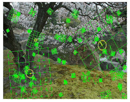
The last phrase immediately prompts thoughts of circumventing such problems: one must either somehow select the points that contribute to the characteristic, or, even better, select some special (key) points and compare them. On this we came up with the idea of ​​comparing images at key points. We can say that we are replacing the image with some model - a set of its key points. Immediately, we note that a point of the depicted object that is most likely to be found on another image of the same object will be called special. A detector is a method for extracting key points from an image. The detector must ensure the invariance of finding the same singular points with respect to image transformations.

The only thing that remains unclear is how to determine which key point of one image corresponds to the key point of another image. After all, after using the detector, you can only determine the coordinates of the singular points, and they are different on each image. This is where the descriptors come in. A descriptor is an identifier of a key point that distinguishes it from the rest of the mass of special points. In turn, descriptors must ensure the invariance of finding correspondence between singular points with respect to image transformations.

As a result, we obtain the following scheme for solving the image matching problem:
1. Key points and their descriptors are highlighted on the images.
2. By coincidence of descriptors, key points corresponding to each other are highlighted.
3. Based on a set of coincident key points, a model for transforming images is built using which you can get another from one image.

At each stage, there are problems and various methods for solving them, which introduces a certain arbitrariness in the solution of the original problem. Next, we will consider the first part of the solution, namely, the allocation of singular points and their descriptors using the SIFT (Scale Invariant Feature Transform) method. Basically, the algorithm of the SIFT method will be described, and not why this algorithm works, and looks exactly like that.

Lastly, we list some transformations with respect to which we would like to obtain invariance:
1) displacements
2) rotation
3) scale (the same object can be of different sizes in different images)
4) changes in brightness
5) changes in camera position

Invariance with respect to the last three transformations cannot be fully obtained, but at least partially it would not be bad to do so.

Finding Special Points

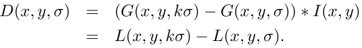
The main point in the detection of singular points is the construction of the pyramid of Gaussian (Gaussian) and differences of Gaussian (Difference of Gaussian, DoG). The Gaussian (or image blurred by a Gaussian filter) is the image. Here L is the value of the Gaussian at the point with coordinates (x, y), and sigma is the blur radius. G is the Gaussian core, I is the value of the original image, * is the convolution operation. Gaussian difference is an image obtained by pixel-by-pixel subtraction of one Gaussian source image from a Gaussian with a different radius.








In a nutshell, let's talk about scalable spaces. Scalable image space is a set of various versions of the original image smoothed by some filter. It is proved that the Gaussian scalable space is linear, invariant with respect to shifts, rotations, and scale, not shifting local extrema, and has the property of semigroups. It is important for us that a different degree of image blurring by a Gaussian filter can be taken as the original image taken at a certain scale.

In general, scale invariance is achieved by finding key points for the original image taken at different scales. To do this, a Gaussian pyramid is built: the entire scalable space is divided into some sections - octaves, and the part of the scalable space occupied by the next octave is two times larger than the part occupied by the previous one. In addition, when moving from one octave to another, resampling of the image is done, its size is halved. Naturally, each octave spans an infinite number of Gaussian images, so only a certain number N of them is built, with a certain step along the blur radius. With the same step, two additional Gaussians are being completed (a total of N + 2 is obtained) that go beyond the octave. Further it will be seen why this is necessary.

In parallel with the construction of the pyramid of Gaussians, a pyramid of differences of Gaussians is constructed, consisting of the differences of neighboring images in the pyramid of Gaussians. Accordingly, the number of images in this pyramid will be N + 1. The figure on the left shows the pyramid of the Gaussians, and on the right - their differences. It is shown schematically that each difference is obtained from two neighboring Gaussians, the number of differences is one less than the number of Gaussians, when moving to the next octave, the image size is halved After the construction of the pyramids, the task remains small. We will consider a point singular if it is a local extremum of the difference of the Gaussians. To search for extrema, we will use the method schematically depicted in the figure







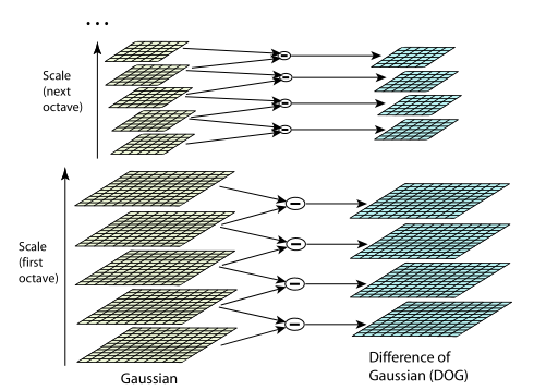
If the value of the difference of the Gaussians at the point marked with a cross is greater (less) than all the values ​​at the points marked with

round circles , then this point is considered the extremum point. In each image from the DoG pyramid, points of local extremum are searched. Each point of the current DoG image is compared with its eight neighbors and nine neighbors in the DoG, which are one level higher and lower in the pyramid. If this point is larger (less) than all neighbors, then it is taken as a point of local extremum.

I think now it should be clear why we needed “extra” images in an octave. In order to check for extremum points N'e the image in the DoG pyramid, you need to have N + 1'e. And in order to get N + 1'e in the DoG pyramid, you must have N + 1'e and N + 2'e images in the Gaussian pyramid. Following the same logic, we can say that it is necessary to build the 0th image (for checking the 1st) in the DoG pyramid and two more in the Gaussian pyramid. But remembering that the 1st image in the current octave has the same scale as the N'e in the previous one (which should already be checked), we can relax a bit and read on :)

Specification of singular points

Oddly enough, in the previous paragraph, the search for key points is not over. The next step will be a couple of checks on the suitability of the extremum for the key role.

First of all, the coordinates of the singular point are determined with subpixel accuracy. This is achieved by approximating the DoG function by the second-order Taylor polynomial taken at the point of the calculated extremum. Here D is the DoG function, X = (x, y, sigma) is the displacement vector relative to the decomposition point, the first DoG derivative is the gradient, the second DoG derivative is the Hessian matrix. The extremum of the Taylor polynomial is found by calculating the derivative and equating it to zero. As a result, we obtain the offset of the point of the calculated extremum, relatively accurate








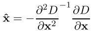
All derivatives are calculated by finite difference formulas. As a result, we get a SLAE of dimension 3x3, relative to the components of the vector X ^.

If one of the components of the vector X ^ is greater than 0.5 * grid_step_ in this_direction, then this means that the extremum point was actually calculated incorrectly and you need to move to the neighboring point in the direction of the indicated components. For a neighboring point, everything repeats again. If in this way we went beyond the octave, then this point should be excluded from consideration.

When the position of the extremum point is calculated, the DoG value itself is checked for smallness at this point by the formula. If this check does not pass, then the point is excluded as a point with low contrast.





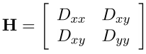
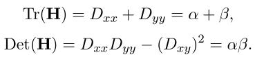
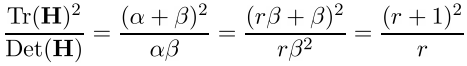
Finally, the last check. If a particular point lies on the boundary of an object or is poorly lit, then such a point can be excluded from consideration. These points have a large bend (one of the components of the second derivative) along the boundary and small in the perpendicular direction. This large bend is determined by the Hessian matrix H. An H of size 2x2 is suitable for testing. Let Tr (H) be the trace of the matrix, and Det (H) be its determinant. Let r be the ratio of the larger bend to the smaller, then the point is further considered if

Finding a Cue Point Orientation

After we make sure that some point is the key, we need to calculate its orientation. As will be seen later, a point can have several directions.

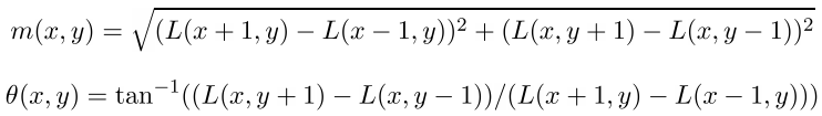
The direction of the key point is calculated based on the direction of the gradients of the points adjacent to the singular. All gradient calculations are performed on the image in the Gaussian pyramid, with the scale closest to the scale of the key point. For reference: the magnitude and direction of the gradient at the point (x, y) are calculated by the formulas m is the magnitude of the gradient, theta is its direction




First, we define the window (neighborhood) of the key point at which the gradients will be considered. In essence, this will be the window required for convolution with the Gaussian core, and it will be round and the blur radius for this core (sigma) is 1.5 * key_point_scale. For the Gaussian kernel, the so-called “three sigma” rule applies. It consists in the fact that the value of the Gaussian nucleus is very close to zero at a distance exceeding 3 * sigma. Thus, the radius of the window is defined as [3 * sigma].

We find the direction of the key point from the histogram of the O directions. The histogram consists of 36 components that uniformly cover the gap of 360 degrees, and it is formed as follows: each point of the window (x, y) makes a contribution equal to m * G (x, y, sigma ), into that component of the histogram that covers the gap containing the gradient direction theta (x, y).

The direction of the key point lies in the gap covered by the maximum component of the histogram. The values ​​of the maximum component (max) and two neighboring components are interpolated by a parabola, and the maximum point of this parabola is taken as the direction of the key point. If there are more components in the histogram with values ​​of at least 0.8 * max, then they are likewise interpolated and additional directions are assigned to the key point.

Building descriptors

Now let's go directly to the descriptors. The earlier definition says what the descriptor should do, but not what it is. In principle, a descriptor can be any object (as long as it copes with its functions), but usually a descriptor is some information about the neighborhood of a key point. This choice was made for several reasons: distortion effects have a smaller effect on small areas, some changes (changing the position of an object in the picture, changing a scene, overlapping one object with another, rotation) may not affect the descriptor at all.

In the SIFT method, the descriptor is a vector. Like the direction of the key point, the handle is calculated on the Gaussian closest in scale to the key point, and based on the gradients in a certain window of the key point. Before calculating the descriptor, this window is rotated by the angle of direction of the key point, thereby achieving invariance with respect to rotation. First, let's look at the figure



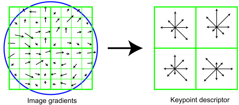
Here, a part of the image (left) and (right) is schematically shown. The descriptor obtained on its basis. First, let's look to the left. Here you can see the pixels indicated by small squares. These pixels are taken from the square window of the descriptor, which in turn is divided into four more equal parts (hereinafter we will call them regions). A small arrow in the center of each pixel indicates the gradient of that pixel. Interestingly, the center of this window is between the pixels. It should be chosen as close as possible to the exact coordinates of the key point. The last detail that can be seen is a circle denoting a convolution window with a Gaussian core (similar to a window for calculating the direction of a key point). For this kernel, sigma is defined equal to half the width of the handle window.

Now let's look to the right. Here we can see a schematically depicted descriptor of a singular point, dimension 2x2x8. The first two digits in the dimension value are the number of regions horizontally and vertically. Those squares that covered a certain region of pixels on the left of the images on the right cover histograms built on the pixels of these regions. Accordingly, the third digit in the dimension of the descriptor means the number of components of the histogram of these regions. The histograms in the regions are calculated in the same way as the histogram of directions with three small but:
1. Each histogram also covers a 360-degree section, but divides it into 8 parts
2. The value of the Gaussian kernel, which is common for the entire descriptor, is taken as the weight coefficient ( this has already been said)
3. The trilinear interpolation coefficients are taken as one more weight coefficients.

Three real coordinates (x, y, n) can be assigned to each gradient in the descriptor window, where x is the horizontal distance to the gradient, y is the vertical distance, n is the distance to the gradient direction in the histogram (meaning the corresponding histogram of the descriptor into which this gradient contributes). The reference point is the lower left corner of the descriptor window and the initial value of the histogram. For single segments, we take the horizontal and vertical sizes of the regions for x and y, respectively, and the number of degrees in the histogram component for n. The coefficient of trilinear interpolation is determined for each coordinate (x, y, n) of the gradient as 1-d, where d is the distance from the coordinate of the gradient to the middle of the unit interval in which this coordinate fell.

The cue point descriptor consists of all the histograms received. As already mentioned, the dimension of the descriptor in figure 32 is the component (2x2x8), but in practice, descriptors of dimension 128 are used (4x4x8).

The resulting descriptor is normalized, after which all its components, whose value is greater than 0.2, are trimmed to 0.2 and then the descriptor is normalized again. As such, the descriptors are ready for use.

Last word and literature

SIFT descriptors are not without flaws. Not all received points and their descriptors will meet the requirements. Naturally, this will affect the further solution of the problem of image matching. In some cases, a solution may not be found, even if it exists. For example, when searching for affine transformations (or a fundamental matrix) from two images of a brick wall, a solution may not be found due to the fact that the wall consists of repeating objects (bricks) that make descriptors of different key points similar to each other. Despite this circumstance, these descriptors work well in many practically important cases.

Plus, this method is patented.

The article describes an example scheme of the SIFT algorithm. If you are interested in why this algorithm is what it is and why it works, as well as the rationale for choosing the values ​​of some parameters taken in the article “from the ceiling” (for example, the number 0.2 in the normalization of the descriptor), then you should refer to the source of
David G. Lowe “Distinctive image features from scale-invariant keypoints”

Another article repeating the main content of the previous one. It details the details of
Yu Meng's Implementing the Scale Invariant Feature Transform (SIFT) Method.