Charts in LaTeX

ftynse January 24, 2010 at 17:12

Many often encounter the need to create various diagrams, graphs, trees for convenient presentation of information. This issue may be especially important when creating presentations. Most office suites offer the ability to create beautiful diagrams using an interactive interface. And if you need to create a large chart? Or write mathematical formulas in it? Focus on the content, not the design and layout of the elements on the screen?

The benefits of using LaTeX have been discussed many times . As well as methods for creating presentations using beamer and vector graphicsfrom the PGF / Tikz package. But is it possible to get diagrams in LaTeX that are not inferior in appearance to those obtained in large and complex packages? One way is suggested below.

Start

First, we need LaTeX ( MiKTeX is suitable for Windows , TeXlive is suitable for Linux or Mac ), as well as beamer and tikz packages . Both are included with the MiKTeX. You can download the latest versions either from the project pages or from CTAN . It will also require basic knowledge of LaTeX, and the use of these packages in it. Since beamer is focused on the use of pdflatex, it will be used mainly PDF.

Simple chart

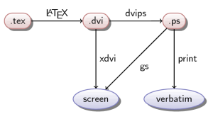
Let's try to make a small and simple diagram. As an example, let's take a sequential conversion of formats when running LaTeX: .tex> .dvi> .ps> .pdf . Suppose we already have a document in which to place this diagram. In the preamble, we connect the tikz package and connect the necessary libraries. In this case, we need positioning and arrows, which are needed to position the elements relative to each other and draw arrows between them, respectively.

\usepackage{tikz} \usetikzlibrary{positioning,arrows}

It should be noted that when listing library names separated by commas, spaces are not allowed. This is due to the fact that tikz substitutes the string completely as part of the library file name.
In the right place in the document, add the tikzpicture environment, inside which the tikz commands are listed. Each command must end with a semicolon. Commands can be nested, for example, to create a signed arrow or children. General command syntax:

\command [parameters] (name) {contents} arguments;

Where

command - the command itself;
parameters - command parameters separated by commas;
name - name of the created object;
contents - content of the object (may include other objects);
arguments - arguments, such as waypoints or sizes, as well as other commands (but without a backslash).

All parts except the team itself are optional. There are hundreds of teams in tikz, path and node will be interesting for us.
The \ path command creates a "path" in the terminology of vector graphics. As a parameter, it is indicated what exactly should be done with this circuit:

draw - only draw an outline;
fill - only fill;
fill, draw - draw a path and fill;
use as bounding box - use the outline as the size limit for the image.

Also indicate the presence and direction of the arrows <-, ->, <->, color, line thickness and other parameters, a complete list can be found in the package documentation.
The arguments are the coordinates through which the contour should pass. There are many options for setting coordinates in tikz:

relative coordinates of the point (1,5);
real on the sheet, in all LaTeX formats (10pt, 3mm);
the use of polar and even the introduction of its own coordinate system;
relative to the previous point ++ (0,1);
relative to the starting point + (- 1,2);
relative to a named object (name).

The points between which you want to draw a line are separated by the operator -. The most suitable LaTeX ideology is positioning relative to objects. For example, to draw a connection between the edges of foo and bar objects, just run the command

\path (foo) edge (bar);

The \ node command creates a node (or object), usually containing some text. Its parameters can be text style, color, information about the presence, shape and color of outlines, location relative to other objects, and many others. You can locate a node in a specific place with coordinates (x, y) using the argument at (x, y). But the most interesting is the location relative to other objects provided by the positioning library. To use it, it is enough to indicate in the parameters in which direction relative to another object the given one should be. for instance

\node (foo) {foo}; \node[right of=foo] (bar) {bar};

For more information, see the documentation. The above is enough to create the first simple diagram. It should have 4 objects, and 3 arrows between them. The implementation looks like this

\node (tex) {.tex}; \node[right of=tex] (dvi) {.dvi}; \node[right of=dvi] (ps) {.ps}; \node[right of=ps] (pdf) {.pdf}; \path[->] (tex) edge (dvi); \path[->] (dvi) edge (ps); \path[->] (ps) edge (pdf);

Improving the chart

We already got the first picture, but it doesn’t look at all: a displaced line of text, lack of frames around the text, objects too close. And this instead of beautiful pictures with gradients and transparency? The diagram is definitely worth improving, and for this we will use the task of styles. The style is set using the command

\tikzstyle{name} = [parameters]

The style name can then be passed as a parameter to another command. For further work, we will also need to connect the shapes and shadows libraries. A good figure for the text would be a rounded rectangle, which is available in the library. For it, you will additionally need to describe the background and outline. Before doing this, let's look at how to set colors in tikz.
The color can be specified by the name of the predefined in LaTeX and the package xcolor. You can also define your RGB color using the command

\definecolor{name}{rgb}{0.5,0.5,0.5}

RGB components are indicated with a comma and their number is from 0 to 1. Or in other systems, which can be read more in the documentation of the xcolor package. Predefined colors can also be mixed. The syntax for this operation is as follows:

color1!percent!color2

The result is a color containing percent% of the first color and (100-percent)% of the second. If the second is not specified, the default color is white. Mixing colors can be repeated without preserving the intermediate color, for example

red!50!black!50!white

First, a color of 50% red and 50% black will be obtained, and then the result is mixed with 50% white. The resulting red and black colors will be 25% each.

Now we can go directly to the task of style

\tikzstyle{format} = [rounded rectangle, thick, minimum size=1cm, draw=red!50!black!50, top color=white, bottom color=red!50!black!20, font=\itshape, drop shadow]

This style prescribes to draw a rectangle with rounded edges, a bold contour line with the color red! 50! Black! 50, fill it using a gradient from top to bottom from white to red! 50! Black! 20, with a shadow, print the inner text in italics.
Next, we should align the baseline of the text. To do this, we first understand why it turned out to be biased. The words "tex", "ps" and "pdf" have different heights, and accordingly were centered differently inside the object. Thus, explicitly specifying the height of the text should solve this problem.
The tikzpicture environment also allows you to set parameters that apply to all teams within this environment. We take advantage of this and set the thickness of the communication line, the minimum distance between objects and the text height parameters in it.

\begin{tikzpicture}[thick, node distance=2cm, text height=1.5ex, text depth=.25ex] \node[format] (tex) {.tex}; \node[format,right of=tex] (dvi) {.dvi}; \node[format,right of=dvi] (ps) {.ps}; \node[format,right of=ps] (pdf) {.pdf}; \path[->] (tex) edge (dvi); \path[->] (dvi) edge (ps); \path[->] (ps) edge (pdf); \end{tikzpicture}

We complicate the task

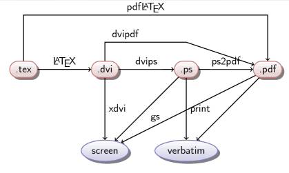
Now that we have an acceptable version of a simple diagram, we will try to complicate the task. We add to this diagram the ways of presenting data (on screen and printed) and the possibility of conversion without intermediate formats. Since there will be many lines on the diagram, it is worth signing them.
Define a different node style for the way data is presented. Let it be an ellipse with a blue gradient from top to bottom, a dark blue outline and shadow. The style description will be similar to the previous one.

\tikzstyle{format} = [ellipse, thick, minimum size=1cm, draw=blue!50!black!50, top color=white, bottom color=blue!50!black!20, drop shadow]

But when adding additional lines, another problem arises. If you set the path from (tex) to (pdf), tikz by default will draw it in a straight line, which does not suit us at all. Unfortunately, the package is not yet able to use graphviz features, so you have to describe the path around the elements yourself. For this, we will use the relative path specification.

\path[->, draw] (tex) -- +(0,2) -| (pdf); \path[->, draw] (dvi) -- ++(0,1) -- ++(3,0) -- (pdf);

The first contour starts from the node (tex) and rises 2 relative units up. Then it continues to the right until the formation of a perpendicular to the node (pdf) and lowers to it. The second circuit starts from the node (dvi), rises by 1 unit, goes right 3 units from the previous point, and goes in a straight line to the node (pdf). To add labels to the contours, use the nested commands and add a node to the contour:

\path[->, draw] (tex) -- +(0,2) -| node[near start] {pdf\LaTeX} (pdf);

But this command will add an object so that the centers of the contour and the node coincide. The text will be crossed out by the line of communication. To prevent this from happening in the tikzpicture environment, we will specify the auto positioning option for auto signatures. Now the description of our diagram will take the form

\begin{tikzpicture}[thick, node distance=3cm, text height=1.5ex, text depth=.25ex, auto] \node[format] (tex) {.tex}; \node[format,right of=tex] (dvi) {.dvi}; \node[format,right of=dvi] (ps) {.ps}; \node[format,right of=ps] (pdf) {.pdf}; \node[medium,below of=dvi] (screen) {screen}; \node[medium,below of=ps] (verbatim) {verbatim}; \path[->] (tex) edge node {\LaTeX} (dvi); \path[->] (dvi) edge node {dvips}(ps); \path[->] (ps) edge node {ps2pdf} (pdf); \path[->] (dvi) edge node {xdvi} (screen); \path[->] (ps) edge node[near start] {gs} (screen); \path[->] (pdf) edge (screen); \path[->] (ps) edge node {print} (verbatim); \path[->] (pdf) edge (verbatim); \path[->, draw] (tex) -- +(0,2) -| node[near start] {pdf\LaTeX} (pdf); \path[->, draw] (dvi) -- ++(0,1) -- node[near start] {dvipdf} ++(3,0) -- (pdf); \end{tikzpicture}

Use in presentation

The resulting diagram can be used as a static picture in an article or description. But presentations often require chart objects to appear in a specific order. LaTeX uses the beamer package to create presentations. His work is built around the concept of overlays - different representations of the same slide. We already wrote about the use of beamer, so let's recall the specification of overlays. They can be added to almost any LaTeX team, and tikz teams are no exception. Therefore, any illustrations obtained using this package are easily divided into parts and integrated with beamer. However, now the commands are not very convenient for adding overlays. If you want the object to appear simultaneously and all its connections with existing ones, you will have to add specifications to each of the teams. It would be more logical to arrange the commands sequentially according to the time of appearance on the slide. Here comes the opportunity to group the teams, which was mentioned at the very beginning. In the \ path command, you can specify the nodes that it will connect. Thus, we can do one team for each overlay.

\begin{frame} \frametitle{\LaTeX workflow} \begin{tikzpicture}[thick, node distance=3cm, text height=1.5ex, text depth=.25ex, auto] \path[use as bounding box] (-1,0) rectangle (10,-2); \path[->]<1-> node[filename] (tex) {.tex}; \path[->]<2-> node[filename, right of=tex] (dvi) {.dvi} (tex) edge node {\LaTeX} (dvi); \path[->]<3-> node[display, below of=dvi] (screen) {screen} (dvi) edge node {xdvi} (screen); \path[->]<4-> node[filename, right of=dvi] (ps) {.ps} (dvi) edge node {dvips} (ps); \path[->]<5-> (ps) edge node {gs} (screen); \path[->]<6-> node[display, below of=ps] (verbatim) {verbatim} (ps) edge node {print} (verbatim); \path[->]<7-> node[filename, right of=ps] (pdf) {.pdf} (ps) edge node {ps2pdf} (pdf); \path[->]<8-> (pdf) edge (screen) edge (verbatim); \path[->, draw]<9-> (tex) -- +(0,2) -| node[near start] {pdf\LaTeX} (pdf); \path[->, draw]<10-> (dvi) -- ++(0,1) -- node[near start] {dvipdf} ++(3,0) -- (pdf); \end{tikzpicture} \end{frame}