July 10, 2019 at 22:53
How to choose a random number from 1 to 10
- Transfer
Imagine that you need to generate a uniformly distributed random number from 1 to 10. That is, an integer from 1 to 10 inclusive, with an equal probability (10%) of each occurrence. But, say, without access to coins, computers, radioactive material, or other similar sources of (pseudo) random numbers. You only have a room with people.
Suppose there are a little over 8500 students in this room.
The simplest thing is to ask someone: “Hey, choose a random number from one to ten!”. The man replies: "Seven!". Excellent! Now you have a number. However, you begin to wonder if it is evenly distributed.
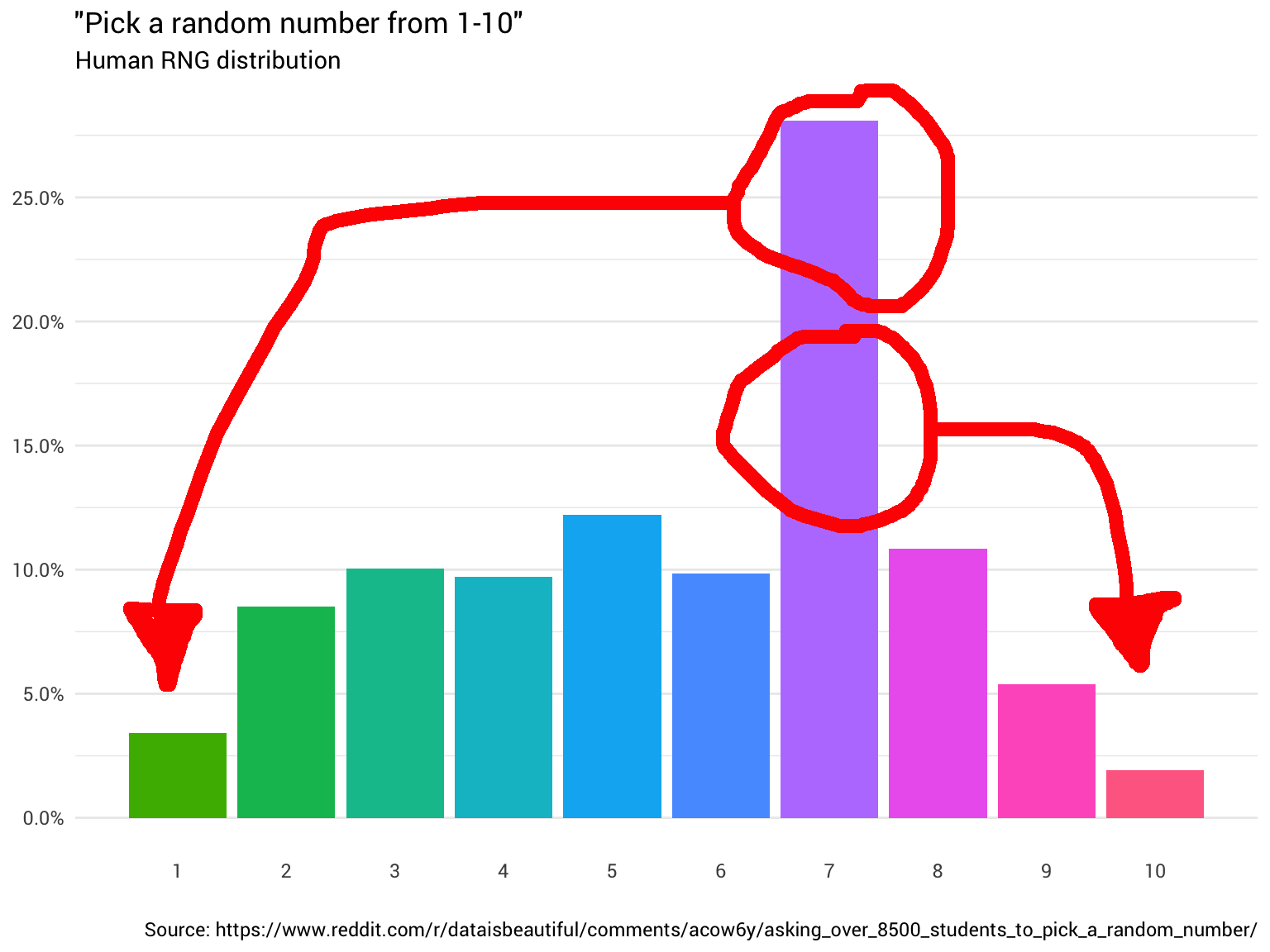
So you decided to ask a few more people. You keep asking them and counting their answers, rounding off the fractional numbers and ignoring those who think that the range from 1 to 10 includes 0. In the end, you begin to see that the distribution is not even at all:

Data from Reddit
You slap your forehead. Well, of course , it will not be random. After all, you cannot trust people .
I wish I could find some function that transforms the distribution of the “human RNG” into a uniform distribution ...
Intuition here is relatively simple. You just need to take the mass of distribution from where it is above 10%, and move it to where it is less than 10%. So that all the columns on the chart are at the same level:
In theory, such a function must exist. In fact, there must be many different functions (for permutation). In an extreme case, you can “cut” each column into infinitely small blocks and build a distribution of any shape (like Lego bricks).
Of course, such an extreme example is a bit cumbersome. Ideally, we want to keep as much of the initial distribution as possible (i.e., to make as few shreds and movements as possible).
Well, our explanation above sounds a lot like linear programming . From Wikipedia:
Linear programming (LP, also called linear optimization) is a method for achieving the best result ... in a mathematical model whose requirements are represented by linear relationships ... The standard form is the usual and most intuitive form of describing a linear programming problem. It consists of three parts:
Similarly, the problem of redistribution can be formulated.
We have a set of variables , each of which encodes a fraction of the probability redistributed from an integer
  (1 to 10) to an integer
  (from 1 to 10). Therefore, if
 , then we need to transfer 20% of the answers from seven to one.
We want to limit these variables in such a way that all redistributed probabilities add up to 10%. In other words, for each from 1 to 10:
We can represent these restrictions as a list of arrays in R. Later, we bind them into a matrix.
We must also make sure that the whole mass of probabilities from the initial distribution is preserved. So for everyone in the range from 1 to 10:
As already mentioned, we want to maximize the preservation of the original distribution. This is our objective :
Then we transfer the problem to the solver, for example, to the package
The following redistribution is returned:
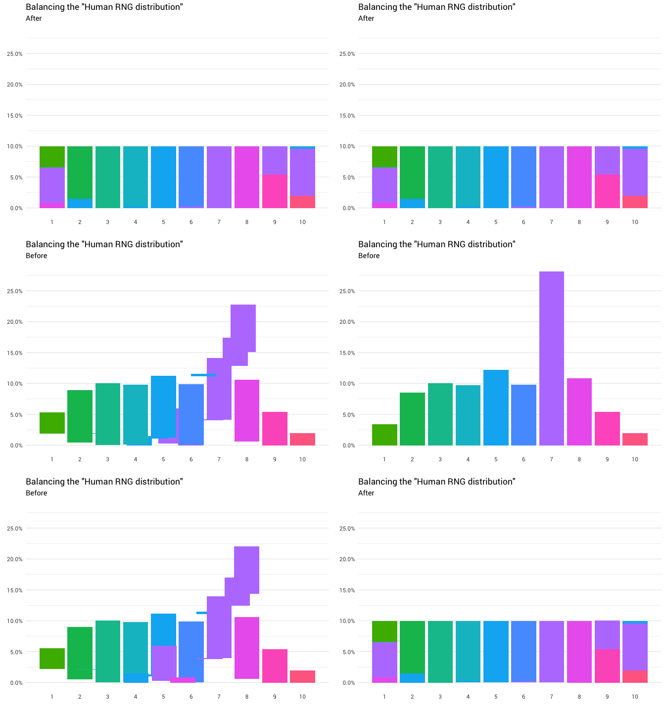
Excellent! Now we have a redistribution function. Let's take a closer look at exactly how the mass moves:

This chart says that in about 8% of cases when someone calls eight as a random number, you need to take the answer as a unit. In the remaining 92% of cases, he remains the eight.
It would be quite simple to solve the problem if we had access to a generator of evenly distributed random numbers (from 0 to 1). But we only have a room full of people. Fortunately, if you are ready to come to terms with a few minor inaccuracies, then you can make a pretty good RNG out of people without asking more than twice.
Returning to our original distribution, we have the following probabilities for each number, which can be used to re-assign any probability, if necessary.
For example, when someone gives us eight as a random number, we need to determine whether this eight should become a unit or not (probability 8%). If we ask another person about a random number, then with a probability of 8.5% he will answer “two”. So if this second number is 2, we know that we must return 1 as a uniformly distributed random number.
Extending this logic to all numbers, we obtain the following algorithm:
Suppose there are a little over 8500 students in this room.
The simplest thing is to ask someone: “Hey, choose a random number from one to ten!”. The man replies: "Seven!". Excellent! Now you have a number. However, you begin to wonder if it is evenly distributed.
So you decided to ask a few more people. You keep asking them and counting their answers, rounding off the fractional numbers and ignoring those who think that the range from 1 to 10 includes 0. In the end, you begin to see that the distribution is not even at all:
library(tidyverse)
probabilities <-
  read_csv("https://git.io/fjoZ2") %>%
  count(outcome = round(pick_a_random_number_from_1_10)) %>%
  filter(!is.na(outcome),
         outcome != 0) %>%
  mutate(p = n / sum(n))
probabilities %>%
  ggplot(aes(x = outcome, y = p)) +
  geom_col(aes(fill = as.factor(outcome))) +
  scale_x_continuous(breaks = 1:10) +
  scale_y_continuous(labels = scales::percent_format(),
                     breaks = seq(0, 1, 0.05)) +
  scale_fill_discrete(h = c(120, 360)) +
  theme_minimal(base_family = "Roboto") +
  theme(legend.position = "none",
        panel.grid.major.x = element_blank(),
        panel.grid.minor.x = element_blank()) +
  labs(title = '"Pick a random number from 1-10"',
       subtitle = "Human RNG distribution",
       x = "",
       y = NULL,
       caption = "Source: https://www.reddit.com/r/dataisbeautiful/comments/acow6y/asking_over_8500_students_to_pick_a_random_number/")
Data from Reddit
You slap your forehead. Well, of course , it will not be random. After all, you cannot trust people .
So what to do?
I wish I could find some function that transforms the distribution of the “human RNG” into a uniform distribution ...
Intuition here is relatively simple. You just need to take the mass of distribution from where it is above 10%, and move it to where it is less than 10%. So that all the columns on the chart are at the same level:
In theory, such a function must exist. In fact, there must be many different functions (for permutation). In an extreme case, you can “cut” each column into infinitely small blocks and build a distribution of any shape (like Lego bricks).
Of course, such an extreme example is a bit cumbersome. Ideally, we want to keep as much of the initial distribution as possible (i.e., to make as few shreds and movements as possible).
How to find such a function?
Well, our explanation above sounds a lot like linear programming . From Wikipedia:
Linear programming (LP, also called linear optimization) is a method for achieving the best result ... in a mathematical model whose requirements are represented by linear relationships ... The standard form is the usual and most intuitive form of describing a linear programming problem. It consists of three parts:
- Linear function to be maximized
- Problem limitations of the following form
- Non-negative variables
Similarly, the problem of redistribution can be formulated.
Presentation of the problem
We have a set of variables
, each of which encodes a fraction of the probability redistributed from an integer (1 to 10) to an integer (from 1 to 10). Therefore, if, then we need to transfer 20% of the answers from seven to one.variables <-
crossing(from = probabilities$outcome,
to = probabilities$outcome) %>%
mutate(name = glue::glue("x({from},{to})"),
ix = row_number())
variables## # A tibble: 100 x 4 ## from to name ix #### 1 1 1 x (1,1) 1 ## 2 1 2 x (1,2) 2 ## 3 1 3 x (1,3) 3 ## 4 1 4 x (1,4) 4 ## 5 1 5 x (1,5) 5 ## 6 1 6 x (1,6) 6 ## 7 1 7 x (1,7) 7 ## 8 1 8 x (1,8) 8 ## 9 1 9 x (1.9) 9 ## 10 1 10 x (1,10) 10 ## # ... with 90 more rows
We want to limit these variables in such a way that all redistributed probabilities add up to 10%. In other words, for each
from 1 to 10:
We can represent these restrictions as a list of arrays in R. Later, we bind them into a matrix.
fill_array <- function(indices,
                       weights,
                       dimensions = c(1, max(variables$ix))) {
  init <- array(0, dim = dimensions)
  if (length(weights) == 1) {
    weights <- rep_len(1, length(indices))
  }
  reduce2(indices, weights, function(a, i, v) {
    a[1, i] <- v
    a
  }, .init = init)
}
constrain_uniform_output <-
  probabilities %>%
  pmap(function(outcome, p, ...) {
    x <-
      variables %>%
      filter(to == outcome) %>%
      left_join(probabilities, by = c("from" = "outcome"))
    fill_array(x$ix, x$p)
  })
We must also make sure that the whole mass of probabilities from the initial distribution is preserved. So for everyone
in the range from 1 to 10:
one_hot <- partial(fill_array, weights = 1)
constrain_original_conserved <-
  probabilities %>%
  pmap(function(outcome, p, ...) {
    variables %>%
      filter(from == outcome) %>%
      pull(ix) %>%
      one_hot()
  })
As already mentioned, we want to maximize the preservation of the original distribution. This is our objective :

maximise_original_distribution_reuse <-
  probabilities %>%
  pmap(function(outcome, p, ...) {
    variables %>%
      filter(from == outcome,
             to == outcome) %>%
      pull(ix) %>%
      one_hot()
  })
objective <- do.call(rbind, maximise_original_distribution_reuse) %>% colSums()
Then we transfer the problem to the solver, for example, to the package
lpSolvein R, combining the created constraints into one matrix:# Make results reproducible...
set.seed(23756434)
solved <- lpSolve::lp(
direction = "max",
objective.in = objective,
const.mat = do.call(rbind, c(constrain_original_conserved, constrain_uniform_output)),
const.dir = c(rep_len("==", length(constrain_original_conserved)),
rep_len("==", length(constrain_uniform_output))),
const.rhs = c(rep_len(1, length(constrain_original_conserved)),
rep_len(1 / nrow(probabilities), length(constrain_uniform_output)))
)
balanced_probabilities <-
variables %>%
mutate(p = solved$solution) %>%
left_join(probabilities,
by = c("from" = "outcome"),
suffix = c("_redistributed", "_original"))The following redistribution is returned:
library(gganimate)
redistribute_anim <-
  bind_rows(balanced_probabilities %>%
            mutate(key   = from,
                   state = "Before"),
            balanced_probabilities %>%
            mutate(key   = to,
                   state = "After")) %>%
  ggplot(aes(x = key, y = p_redistributed * p_original)) +
  geom_col(aes(fill = as.factor(from)),
           position = position_stack()) +
  scale_x_continuous(breaks = 1:10) +
  scale_y_continuous(labels = scales::percent_format(),
                     breaks = seq(0, 1, 0.05)) +
  scale_fill_discrete(h = c(120, 360)) +
  theme_minimal(base_family = "Roboto") +
  theme(legend.position = "none",
        panel.grid.major.x = element_blank(),
        panel.grid.minor.x = element_blank()) +
  labs(title = 'Balancing the "Human RNG distribution"',
       subtitle = "{closest_state}",
       x = "",
       y = NULL) +
  transition_states(
    state,
    transition_length = 4,
    state_length = 3
  ) +
  ease_aes('cubic-in-out')
animate(
  redistribute_anim,
  start_pause = 8,
  end_pause = 8
)
Excellent! Now we have a redistribution function. Let's take a closer look at exactly how the mass moves:
balanced_probabilities %>%
  ggplot(aes(x = from, y = to)) +
  geom_tile(aes(alpha = p_redistributed, fill = as.factor(from))) +
  geom_text(aes(label = ifelse(p_redistributed == 0, "", scales::percent(p_redistributed, 2)))) +
  scale_alpha_continuous(limits = c(0, 1), range = c(0, 1)) +
  scale_fill_discrete(h = c(120, 360)) +
  scale_x_continuous(breaks = 1:10) +
  scale_y_continuous(breaks = 1:10) +
  theme_minimal(base_family = "Roboto") +
  theme(panel.grid.minor = element_blank(),
        panel.grid.major = element_line(linetype = "dotted"),
        legend.position = "none") +
  labs(title = "Probability mass redistribution",
       x = "Original number",
       y = "Redistributed number")
This chart says that in about 8% of cases when someone calls eight as a random number, you need to take the answer as a unit. In the remaining 92% of cases, he remains the eight.
It would be quite simple to solve the problem if we had access to a generator of evenly distributed random numbers (from 0 to 1). But we only have a room full of people. Fortunately, if you are ready to come to terms with a few minor inaccuracies, then you can make a pretty good RNG out of people without asking more than twice.
Returning to our original distribution, we have the following probabilities for each number, which can be used to re-assign any probability, if necessary.
probabilities %>%
  transmute(number = outcome,
            probability = scales::percent(p))
## # A tibble: 10 x 2 ## number probability #### 1 1 3.4% ## 2 2 8.5% ## 3 3 10.0% ## 4 4 9.7% ## 5 5 12.2% ## 6 6 9.8% ## 7 7 28.1% ## 8 8 10.9% ## 9 9 5.4% ## 10 10 1.9%
For example, when someone gives us eight as a random number, we need to determine whether this eight should become a unit or not (probability 8%). If we ask another person about a random number, then with a probability of 8.5% he will answer “two”. So if this second number is 2, we know that we must return 1 as a uniformly distributed random number.
Extending this logic to all numbers, we obtain the following algorithm:
Using this algorithm, you can use a group of people to get something close to a generator of evenly distributed random numbers from 1 to 10!
- Ask a person for a random number,
.
or
:
- Your random number
- If
:
- Ask another person for a random number (
)
- If
(12.2%):
- Your random number 2
- If
(1.9%):
- Your random number 4
- Otherwise, your random number is 5
- If
:
- Ask another person for a random number (
- If
or
(20.7%):
- Your random number 1
- If
or
(16.2%):
- Your random number is 9
- If
(28.1%):
- Your random number is 10
- Otherwise, your random number is 7
- If
:
- Ask another person for a random number (
- If
- Your random number 1
- Otherwise, your random number is 8