On autoregressive estimation of the spectral density of a stationary signal
Methods of spectral estimation of stationary random processes based on the fast Fourier transform (FFT) are well known and widely used in engineering practice. Their disadvantages include, in particular, a high dispersion (low accuracy) of the estimate with an insufficiently long observation interval for the process, which visually usually manifests itself in a strong "indented" graph of the power spectral density (PSD). One of the alternative methods of spectral estimation is the autoregressive method, considered in the example below, which is much less known in engineering practice. In many cases, the method makes it relatively easy to obtain a much better estimate of the PSD (Fig. 1), and sometimes even deeper information about the random process under study.

Fig. 1. Classical and autoregressive evaluation of the PSD of the “short” process.
For demonstration purposes, a discrete-time signal (sequence) x [i] was synthesized. The signal is modeled using an ARMA model (digital filter) simulating the properties of a mechanical system (1) - moving the material point x (t) in a “single-mass” oscillator with parameters m = 1 kg, c = 100 N / m, k = 2, 5 kg / s, and by a force perturbation - Gaussian “white” (taking into account discretization) noise f (t) with a dispersion of 1 N 2 , the sampling interval in time Δt = 0.12 s.

Model built (2). The method of constructing the model has already been considered earlier here . x [i] - 0.6388 · x [i-1] + 0.7408 · x [i-2] = 0.009667 · f [i-1] (2)
Using (2), a sequence of 50 thousand samples was synthesized, for which a generator of a normally distributed random variable randn () of a well-known software environment was used.
After the simulation of the process x [i] is completed, the quantitative parameters of the model (2) are assumed to be unknown - only the process itself and, to some extent, information about the properties of the model in the most general terms are available for research.
A spectral estimation of the 50,000-point sequence was carried out using the Welch method, the segment size was taken equal to 256 samples, the Hamming window and 60% overlap of the segments were applied. The standard deviation of such an estimate, based on the fact that the sequence has a length of about 200 non-overlapping segments, can be roughly estimated as ~ 7%.
Further, assuming that under real conditions in the experiment, a much shorter sequence is available for research, studies were carried out only on the first 500 samples of this signal.
An estimate is obtained by the Welch method with the same parameters. The standard deviation of such an estimate is ~ 70%; a very strong “roughness” of the graph is noticeable (Fig. 2).

Fig.2. Estimation of the “long” and “short” PSDs by the classical method.
Based on the fact that the approximate form of the function (graph) of the PSD process is known to us (for example, based on the known physical nature of the process - a single-mass oscillator under white noise, or from evaluating similar processes for which longer implementations are available), a decision was made to evaluate using the second-order autoregressive model (AR (2), or = ARMA (2.0)).
Determining the order of the model is a very important point; an error in the order can lead to very gross errors in the estimation results. There are methods that are not yet considered here, helping to determine the order of the model based on only the process being analyzed.
The model parameters were estimated using the well-known Yule-Walker equations for the autoregressive process (slightly modified to slightly simplify the script structure):
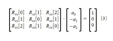
As can be seen from the equations, to determine the parameters, only the first three members of the autoregressive sequence Rxx [0], Rxx [1], are needed Rxx [2], which were estimated from the initial 500-point sequence x [i] by the correlogram method, the standard deviation of this estimate is ~ 4.5%.
(By the way, it can be seen that the "cons" before a 1 , a22 , etc., are extremely uncomfortable. They appeared because of the predominantly “predictive” use of ARMA models in the economy; in earlier “engineering” sources they are not. I already doubt that it was necessary to use such an understanding of AR-coefficients here.
) In practice, the correlation matrix in (3) always has a strict diagonal prevalence | Rxx [0] | > | Rxx [i] |, including due to the presence of observation noises, as a result of which there are no difficulties with its handling (finding a solution (3)).
(To clarify the question of the magnitude of the statistical modeling error, it is interesting to mention, for example, the estimate Rxx [0] = 2.2606e-04 m 2 obtained from 500 samples, in comparison with the correlogram obtained dispersion estimates from 50,000 samples, = 2.4238e-04 m 2and the estimate for the integrand PSD area obtained by the Welch method for 50,000 samples (Fig. 2), = 2.4232e-04 m 2 )
After substituting the found estimates Rxx [i] we have:
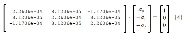
The following model parameters are determined a 0 = 11325.9; a 1 = 7090.1; a 2 = -8411.5; As can be seen from (3), the dispersion of the hypothetical incoming white noise was set = 1 here, determining instead of it the gain a 0 . Autoregressive estimation of PSD is constructed by the Fourier transform over a sequence of coefficients a 0 , a 1 , a 2 :

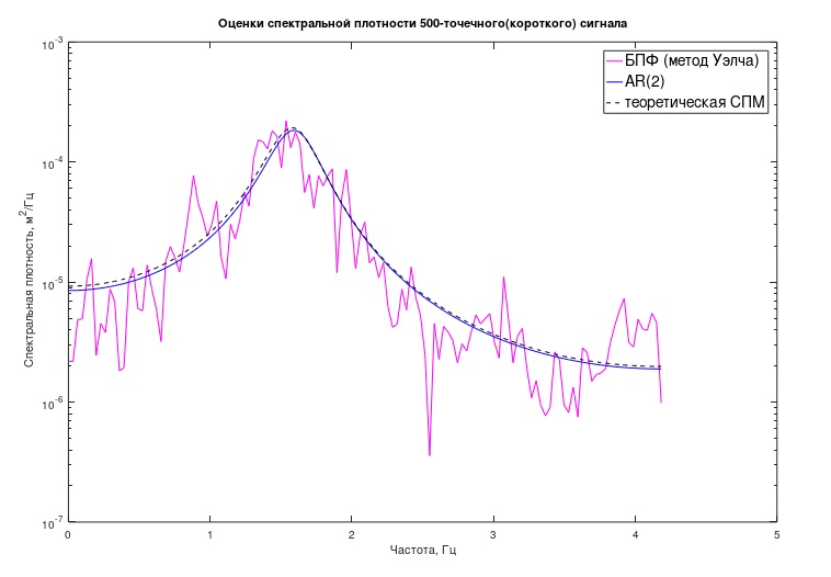
Fig.3 Classical and autoregressive estimation of PSD of a “short” process
In the same way, according to an expression similar to (5), the “theoretical” schedule of the PSD was earlier constructed, only the model coefficients there, of course, were taken different (from (2)).
It can be seen from the graph that the AR estimate of the PSD turned out to be very close to the theoretically expected one. In addition to the graph, it is possible to try to evaluate some analytical characteristics of the process and the associated mechanical system. In this case, these are the "poles" of the model, numerically characterizing the frequencies of the "resonant" peaks of the model and the associated "quality factors".
From (5) we find the relation for searching the discontinuities of the transfer function of our model using the Laplace transform (replacing jω by λ = -ε + jω):

For the obtained AR model in this way, λ 1,2= -1.5427 ± j · 10.1514, which is very close to the original model used to generate the process
λ 1,2theor = -1.2500 ± j · 9.9216 (i.e., the positions of the resonance peak, respectively, 1,615 Hz (in theory) and 1,579 Hz (determined )).
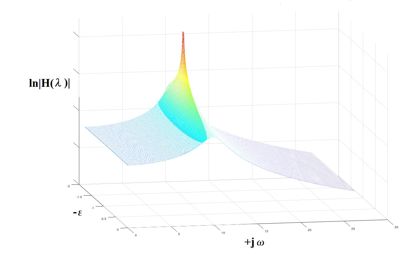
Fig. 4 On the concept of “poles”
A few comments and recommendations in conclusion.
Fig. 1. Classical and autoregressive evaluation of the PSD of the “short” process.
For demonstration purposes, a discrete-time signal (sequence) x [i] was synthesized. The signal is modeled using an ARMA model (digital filter) simulating the properties of a mechanical system (1) - moving the material point x (t) in a “single-mass” oscillator with parameters m = 1 kg, c = 100 N / m, k = 2, 5 kg / s, and by a force perturbation - Gaussian “white” (taking into account discretization) noise f (t) with a dispersion of 1 N 2 , the sampling interval in time Δt = 0.12 s.
Model built (2). The method of constructing the model has already been considered earlier here . x [i] - 0.6388 · x [i-1] + 0.7408 · x [i-2] = 0.009667 · f [i-1] (2)
Using (2), a sequence of 50 thousand samples was synthesized, for which a generator of a normally distributed random variable randn () of a well-known software environment was used.
After the simulation of the process x [i] is completed, the quantitative parameters of the model (2) are assumed to be unknown - only the process itself and, to some extent, information about the properties of the model in the most general terms are available for research.
A spectral estimation of the 50,000-point sequence was carried out using the Welch method, the segment size was taken equal to 256 samples, the Hamming window and 60% overlap of the segments were applied. The standard deviation of such an estimate, based on the fact that the sequence has a length of about 200 non-overlapping segments, can be roughly estimated as ~ 7%.
Further, assuming that under real conditions in the experiment, a much shorter sequence is available for research, studies were carried out only on the first 500 samples of this signal.
An estimate is obtained by the Welch method with the same parameters. The standard deviation of such an estimate is ~ 70%; a very strong “roughness” of the graph is noticeable (Fig. 2).
Fig.2. Estimation of the “long” and “short” PSDs by the classical method.
Based on the fact that the approximate form of the function (graph) of the PSD process is known to us (for example, based on the known physical nature of the process - a single-mass oscillator under white noise, or from evaluating similar processes for which longer implementations are available), a decision was made to evaluate using the second-order autoregressive model (AR (2), or = ARMA (2.0)).
Determining the order of the model is a very important point; an error in the order can lead to very gross errors in the estimation results. There are methods that are not yet considered here, helping to determine the order of the model based on only the process being analyzed.
The model parameters were estimated using the well-known Yule-Walker equations for the autoregressive process (slightly modified to slightly simplify the script structure):
As can be seen from the equations, to determine the parameters, only the first three members of the autoregressive sequence Rxx [0], Rxx [1], are needed Rxx [2], which were estimated from the initial 500-point sequence x [i] by the correlogram method, the standard deviation of this estimate is ~ 4.5%.
(By the way, it can be seen that the "cons" before a 1 , a22 , etc., are extremely uncomfortable. They appeared because of the predominantly “predictive” use of ARMA models in the economy; in earlier “engineering” sources they are not. I already doubt that it was necessary to use such an understanding of AR-coefficients here.
) In practice, the correlation matrix in (3) always has a strict diagonal prevalence | Rxx [0] | > | Rxx [i] |, including due to the presence of observation noises, as a result of which there are no difficulties with its handling (finding a solution (3)).
(To clarify the question of the magnitude of the statistical modeling error, it is interesting to mention, for example, the estimate Rxx [0] = 2.2606e-04 m 2 obtained from 500 samples, in comparison with the correlogram obtained dispersion estimates from 50,000 samples, = 2.4238e-04 m 2and the estimate for the integrand PSD area obtained by the Welch method for 50,000 samples (Fig. 2), = 2.4232e-04 m 2 )
After substituting the found estimates Rxx [i] we have:
The following model parameters are determined a 0 = 11325.9; a 1 = 7090.1; a 2 = -8411.5; As can be seen from (3), the dispersion of the hypothetical incoming white noise was set = 1 here, determining instead of it the gain a 0 . Autoregressive estimation of PSD is constructed by the Fourier transform over a sequence of coefficients a 0 , a 1 , a 2 :
Fig.3 Classical and autoregressive estimation of PSD of a “short” process
In the same way, according to an expression similar to (5), the “theoretical” schedule of the PSD was earlier constructed, only the model coefficients there, of course, were taken different (from (2)).
It can be seen from the graph that the AR estimate of the PSD turned out to be very close to the theoretically expected one. In addition to the graph, it is possible to try to evaluate some analytical characteristics of the process and the associated mechanical system. In this case, these are the "poles" of the model, numerically characterizing the frequencies of the "resonant" peaks of the model and the associated "quality factors".
From (5) we find the relation for searching the discontinuities of the transfer function of our model using the Laplace transform (replacing jω by λ = -ε + jω):
For the obtained AR model in this way, λ 1,2= -1.5427 ± j · 10.1514, which is very close to the original model used to generate the process
λ 1,2theor = -1.2500 ± j · 9.9216 (i.e., the positions of the resonance peak, respectively, 1,615 Hz (in theory) and 1,579 Hz (determined )).
Fig. 4 On the concept of “poles”
A few comments and recommendations in conclusion.
- The “excessive” (too large) order of the AR model is usually much less dangerous than insufficient, from the point of view of the risk of obtaining a PSD estimate with gross errors.
- As a rule, AR-modeling makes it possible to fairly accurately determine the resonant frequencies jω k and much less accurately determine the widths of the corresponding “peaks” -ε k
- ARMA - the model can turn out to be much smaller order (size) than the AR-model, which seems to be aimed at to improve the accuracy of the model, according to many sources. However, evaluating the MA-part of the model is much more difficult and may generally include the first step in obtaining a large-order AR-model in order to further transform it into the MA-part. In connection with these sources, an alternative opinion is also expressed about the advisability of using exactly AR-models for spectral estimation, albeit of a higher order.
- For very short, as well as for non-stationary processes, instead of the matrix of estimates of the autocorrelation function, the covariance matrix is usually used in (3).
- For a detailed study of the issue of autoregressive spectral estimation, S.L. Marple ml. “Digital spectral analysis and its applications”, M., Mir, 1990