Neural Quantum States - Representation of a wave function by a neural network
In this article, we will consider the unusual application of neural networks in general and limited Boltzmann machines in particular for solving two complex problems of quantum mechanics - finding the ground state energy and approximating the wave function of a many-body system.
We can say that this is a free and simplified retelling of an article [2], published in Science in 2017 and some subsequent works. I did not find popular scientific expositions of this work in Russian (and only this one of the English versions ), although it seemed to me very interesting.
Today, there is an opinion among specialists in deep learning that limited
Boltzmann machines (hereinafter - OMB) is an outdated concept that is practically not applicable in real tasks. However, in 2017, an article [2] appeared in Science that showed the very efficient use of OMB for problems of quantum mechanics.
The authors noticed two important facts that may seem obvious, but they had never occurred to anyone before:
Well and further the authors said: let our system be completely described by the wave function, which is the root of the OMB energy, and the OMB inputs are the characteristics of our state of the system (coordinates, spins, etc.):
where s are the characteristics of the state (for example, backs), h are the outputs of the hidden layer of OMB, E is the energy of OMB, Z is the normalization constant (statistical sum).
That's it, the article in Science is ready, then only a few small details remain. For example, it is necessary to solve the problem of non-computable partition function due to the huge size of the Hilbert space. And Tsybenko’s theorem tells us that a neural network can approximate any function, but it doesn’t say at all how to find a suitable set of network weights and offsets for this. Well, and as usual, the fun begins here.
Now there are quite a few modifications of the original approach, but I will only consider the approach from the original article [2].
In our case, the training task will be as follows: to find an approximation of the wave function that would make the state with minimum energy the most probable. This is intuitively clear: the wave function gives us the probability of a state, the eigenvalue of the Hamiltonian (the energy operator, or even simpler, energy - this understanding is enough in the framework of this article) for the wave function is energy. Everything is simple.
In reality, we will strive to optimize another quantity, the so-called local energy, which is always greater than or equal to the energy of the ground state:
here Is our condition
  - all possible states of the Hilbert space (in reality we will consider a more approximate value),
  Is the matrix element of the Hamiltonian. Heavily dependent on the specific Hamiltonian, for example, for the Ising model, this is just
 , if
, if  , and
, and  in all other cases. Do not stop here now; it is important that these elements can be found for various popular Hamiltonians.
An important part of the approach from the original article was the sampling process. A modified variation of the Metropolis-Hastings algorithm was used . The bottom line is:
As a result, we obtain a set of random states selected in accordance with the distribution that our wave function gives us. You can calculate the energy values in each state and the mathematical expectation of energy .
.
It can be shown that the estimate of the energy gradient (more precisely, the expected value of the Hamiltonian) is equal to:
Then we just solve the optimization problem:
As a result, the energy gradient tends to zero, the energy value decreases, as does the number of unique new states in the Metropolis-Hastings process, because by sampling from the true wave function we will almost always get the ground state. Intuitively, this seems logical.
In the original work, for small systems, the values of the ground state energy were obtained, very close to the exact values obtained analytically. A comparison was made with the well-known approaches to finding the ground state energy, and NQS won, especially considering the relatively low computational complexity of NQS in comparison with the known methods.
One of the authors of the original article [2] with his team developed the excellent NetKet library [3], which contains a very well-optimized (in my opinion) C-kernel, as well as the Python API, which works with high-level abstractions.
The library can be installed via pip. Windows 10 users will have to use Linux Subsystem for Windows.
Let us consider working with the library as an example of a chain of 40 spins taking the values + -1 / 2. We will consider the Heisenberg model, which takes into account neighboring interactions.
NetKet has excellent documentation that allows you to quickly figure out what and how to do. There are many built-in models (backs, bosons, Ising, Heisenberg models, etc.), and the ability to fully describe the model yourself.
All models are presented in graphs. For our chain, the built-in Hypercube model with one dimension and periodic boundary conditions is suitable:
Our Hilbert space is very simple - all spins can take values either +1/2 or -1/2. For this case, the built-in model for spins is suitable:
As I already wrote, in our case the Hamiltonian is the Heisenberg Hamiltonian for which there is a built-in operator:
In NetKet, you can use a ready-made RBM implementation for spins - this is just our case. But in general there are many cars, you can try different ones.
Here alpha is the density of neurons in the hidden layer. For 40 neurons of the visible and alpha 4, there will be 160 of them. There is another way of indicating directly by number. The second command initializes weights randomly from . In our case, sigma is 0.01.
A sampler is an object that will be returned to us by a sample from our distribution, which is given by the wave function on the Hilbert space. We will use the Metropolis-Hastings algorithm described above, modified for our task:
To be precise, the sampler is a trickier algorithm than the one I described above. Here we simultaneously check as many as 12 options in parallel to select the next point. But the principle, in general, is the same.
This describes the optimizer that will be used to update the model weights. According to personal experience working with neural networks in areas that are more “familiar” to them, the best and most reliable option is the good old stochastic gradient descent with a moment (well described here ):
NetKet has training both without a teacher (our case) and with a teacher (for example, the so-called “quantum tomography”, but this is the topic of a separate article). We simply describe the “teachers”, and that’s it:
The variational Monte Carlo indicates how we evaluate the gradient of the function we are optimizing.
We will run the model as follows:
The library is built using OpenMPI, and the script will need to be run something like this:
The results I received are as follows:
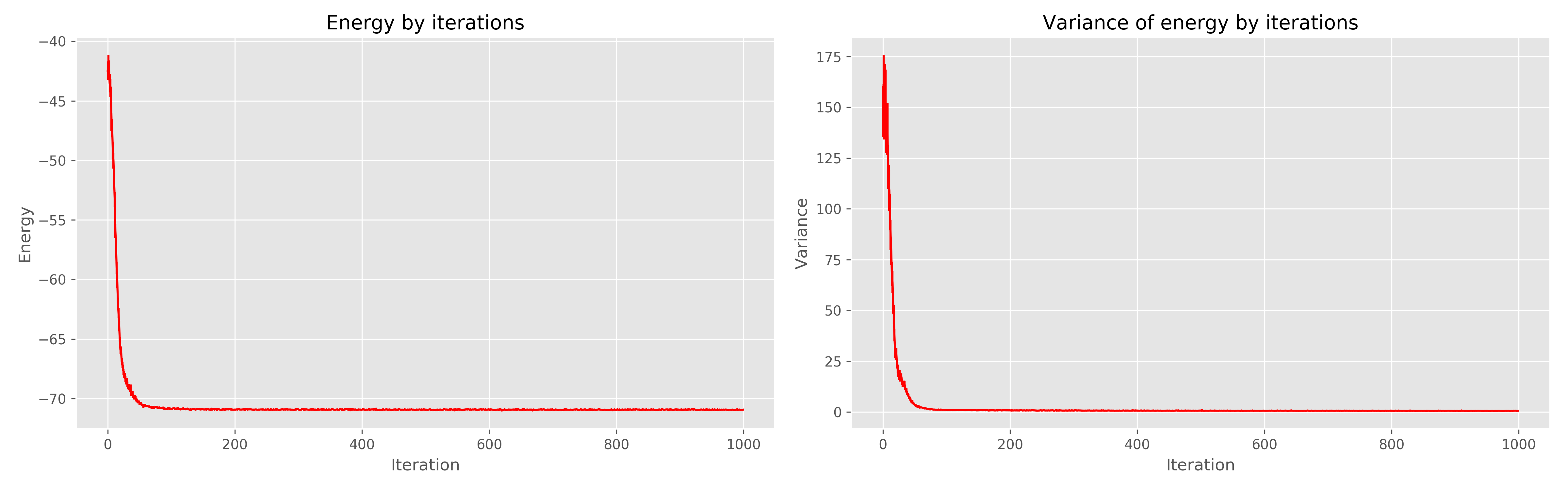
On the left is a graph of energy from the era of learning, on the right is the dispersion of energy from the era of learning.
It can be seen that 1000 eras is clearly redundant, 300 would have been enough. In general, it works very cool, converges quickly.
We can say that this is a free and simplified retelling of an article [2], published in Science in 2017 and some subsequent works. I did not find popular scientific expositions of this work in Russian (and only this one of the English versions ), although it seemed to me very interesting.
Minimum essential concepts from quantum mechanics and deep learning
I want to note right away that these definitions are extremely simplified . I bring them for those for whom the described problem is a dark forest.
A state is simply a set of physical quantities that describe a system. For example, for an electron flying in space it will be its coordinates and momentum, and for a crystal lattice it will be a set of spins of atoms located in its nodes.
The wave function of the system is a complex function of the state of the system. A certain black box that takes an input, for example, a set of spins, but returns a complex number. The main property of the wave function that is important for us is that its square is equal to the probability of this state:
Hilbert space — in our case, such a definition is enough — the space of all possible states of the system. For example, for a system of 40 spins that can take the values +1 or -1, Hilbert space is all possible conditions. For coordinates that can take values
![$ [- \ infty, + \ infty] $](https://habrastorage.org/getpro/habr/formulas/fe4/0d2/e2d/fe40d2e2d2881bf17bd089dde3a06d83.svg) , the dimension of the Hilbert space is infinite. It is the enormous dimension of the Hilbert space for any real systems that is the main problem that does not allow solving equations analytically: in the process there will be integrals / summations over the entire Hilbert space that cannot be calculated “head-on”. A curious fact: for the entire life of the Universe you can meet only a small part of all possible states included in the Hilbert space. This is very well illustrated by a picture from an article about Tensor Networks [1], which schematically depicts the entire Hilbert space and those states that can be met after a polynomial from the characteristic of the complexity of space (number of bodies, particles, spins, etc.)
, the dimension of the Hilbert space is infinite. It is the enormous dimension of the Hilbert space for any real systems that is the main problem that does not allow solving equations analytically: in the process there will be integrals / summations over the entire Hilbert space that cannot be calculated “head-on”. A curious fact: for the entire life of the Universe you can meet only a small part of all possible states included in the Hilbert space. This is very well illustrated by a picture from an article about Tensor Networks [1], which schematically depicts the entire Hilbert space and those states that can be met after a polynomial from the characteristic of the complexity of space (number of bodies, particles, spins, etc.)

A limited Boltzmann machine — if difficult to explain, it is an undirected graphical probabilistic model, the limitation of which is the conditional independence of the probabilities of the nodes of one layer from the nodes of the same layer. If in a simple way, then this is a neural network with an input and one hidden layer. The output values of neurons in the hidden layer can be 0 or 1. The difference from the usual neural network is that the outputs of the hidden layer neurons are random variables selected with probability equal to the value of the activation function:- sigmoid activation function , - offset for the i-th neuron,
  - the weight of the neural network,
  - visible layer. Limited Boltzmann machines belong to the so-called "energy models", since we can express the probability of a particular state of a machine using the energy of this machine:
where v and h are the visible and hidden layers, a and b are the displacements of the visible and hidden layers, W are the weights. Then the probability of the state is representable in the form:
where Z is the normalization term, also called the statistical sum (it is necessary so that the total probability is equal to unity).
A state is simply a set of physical quantities that describe a system. For example, for an electron flying in space it will be its coordinates and momentum, and for a crystal lattice it will be a set of spins of atoms located in its nodes.
The wave function of the system is a complex function of the state of the system. A certain black box that takes an input, for example, a set of spins, but returns a complex number. The main property of the wave function that is important for us is that its square is equal to the probability of this state:

Hilbert space — in our case, such a definition is enough — the space of all possible states of the system. For example, for a system of 40 spins that can take the values +1 or -1, Hilbert space is all
possible conditions. For coordinates that can take values, the dimension of the Hilbert space is infinite. It is the enormous dimension of the Hilbert space for any real systems that is the main problem that does not allow solving equations analytically: in the process there will be integrals / summations over the entire Hilbert space that cannot be calculated “head-on”. A curious fact: for the entire life of the Universe you can meet only a small part of all possible states included in the Hilbert space. This is very well illustrated by a picture from an article about Tensor Networks [1], which schematically depicts the entire Hilbert space and those states that can be met after a polynomial from the characteristic of the complexity of space (number of bodies, particles, spins, etc.)A limited Boltzmann machine — if difficult to explain, it is an undirected graphical probabilistic model, the limitation of which is the conditional independence of the probabilities of the nodes of one layer from the nodes of the same layer. If in a simple way, then this is a neural network with an input and one hidden layer. The output values of neurons in the hidden layer can be 0 or 1. The difference from the usual neural network is that the outputs of the hidden layer neurons are random variables selected with probability equal to the value of the activation function:

- sigmoid activation function , - offset for the i-th neuron, - the weight of the neural network, - visible layer. Limited Boltzmann machines belong to the so-called "energy models", since we can express the probability of a particular state of a machine using the energy of this machine:
where v and h are the visible and hidden layers, a and b are the displacements of the visible and hidden layers, W are the weights. Then the probability of the state is representable in the form:

where Z is the normalization term, also called the statistical sum (it is necessary so that the total probability is equal to unity).
Introduction
Today, there is an opinion among specialists in deep learning that limited
Boltzmann machines (hereinafter - OMB) is an outdated concept that is practically not applicable in real tasks. However, in 2017, an article [2] appeared in Science that showed the very efficient use of OMB for problems of quantum mechanics.
The authors noticed two important facts that may seem obvious, but they had never occurred to anyone before:
- OMB is a neural network that, according to Tsybenko’s universal theorem , can theoretically approximate any function with arbitrarily high accuracy (there are still a lot of restrictions, but you can skip them).
- OMB is a system whose probability of each state is a function of the input (visible layer), weights and displacements of the neural network.
Well and further the authors said: let our system be completely described by the wave function, which is the root of the OMB energy, and the OMB inputs are the characteristics of our state of the system (coordinates, spins, etc.):

where s are the characteristics of the state (for example, backs), h are the outputs of the hidden layer of OMB, E is the energy of OMB, Z is the normalization constant (statistical sum).
That's it, the article in Science is ready, then only a few small details remain. For example, it is necessary to solve the problem of non-computable partition function due to the huge size of the Hilbert space. And Tsybenko’s theorem tells us that a neural network can approximate any function, but it doesn’t say at all how to find a suitable set of network weights and offsets for this. Well, and as usual, the fun begins here.
Model training
Now there are quite a few modifications of the original approach, but I will only consider the approach from the original article [2].
Task
In our case, the training task will be as follows: to find an approximation of the wave function that would make the state with minimum energy the most probable. This is intuitively clear: the wave function gives us the probability of a state, the eigenvalue of the Hamiltonian (the energy operator, or even simpler, energy - this understanding is enough in the framework of this article) for the wave function is energy. Everything is simple.
In reality, we will strive to optimize another quantity, the so-called local energy, which is always greater than or equal to the energy of the ground state:

here
Is our condition - all possible states of the Hilbert space (in reality we will consider a more approximate value), Is the matrix element of the Hamiltonian. Heavily dependent on the specific Hamiltonian, for example, for the Ising model, this is just, if , and in all other cases. Do not stop here now; it is important that these elements can be found for various popular Hamiltonians.Optimization process
Sampling
An important part of the approach from the original article was the sampling process. A modified variation of the Metropolis-Hastings algorithm was used . The bottom line is:
- We start from a random state.
- We change the sign of a randomly selected spin to the opposite (for the coordinates there are other modifications, but they also exist).
- With probability equal to
 , move to a new state.
 - Repeat N times.
As a result, we obtain a set of random states selected in accordance with the distribution that our wave function gives us. You can calculate the energy values in each state and the mathematical expectation of energy
. It can be shown that the estimate of the energy gradient (more precisely, the expected value of the Hamiltonian) is equal to:

Conclusion
This is from a lecture given by G. Carleo in 2017 for Advanced School on Quantum Science and Quantum Technology. There are entries on Youtube.
Denote:
Then:
Denote:

Then:


Then we just solve the optimization problem:
- We sample states from our OMB.
- We calculate the energy of each state.
- Estimate the gradient.
- We update the weight of OMB.
As a result, the energy gradient tends to zero, the energy value decreases, as does the number of unique new states in the Metropolis-Hastings process, because by sampling from the true wave function we will almost always get the ground state. Intuitively, this seems logical.
In the original work, for small systems, the values of the ground state energy were obtained, very close to the exact values obtained analytically. A comparison was made with the well-known approaches to finding the ground state energy, and NQS won, especially considering the relatively low computational complexity of NQS in comparison with the known methods.
NetKet - a library from the "inventors" approach
One of the authors of the original article [2] with his team developed the excellent NetKet library [3], which contains a very well-optimized (in my opinion) C-kernel, as well as the Python API, which works with high-level abstractions.
The library can be installed via pip. Windows 10 users will have to use Linux Subsystem for Windows.
Let us consider working with the library as an example of a chain of 40 spins taking the values + -1 / 2. We will consider the Heisenberg model, which takes into account neighboring interactions.
NetKet has excellent documentation that allows you to quickly figure out what and how to do. There are many built-in models (backs, bosons, Ising, Heisenberg models, etc.), and the ability to fully describe the model yourself.
Count Description
All models are presented in graphs. For our chain, the built-in Hypercube model with one dimension and periodic boundary conditions is suitable:
import netket as nk
graph = nk.graph.Hypercube(length=40, n_dim=1, pbc=True)
Description of Hilbert Space
Our Hilbert space is very simple - all spins can take values either +1/2 or -1/2. For this case, the built-in model for spins is suitable:
hilbert = nk.hilbert.Spin(graph=graph, s=0.5)
Description of the Hamiltonian
As I already wrote, in our case the Hamiltonian is the Heisenberg Hamiltonian for which there is a built-in operator:
hamiltonian = nk.operator.Heisenberg(hilbert=hilbert)
Description of RBM
In NetKet, you can use a ready-made RBM implementation for spins - this is just our case. But in general there are many cars, you can try different ones.
nk.machine.RbmSpin(hilbert=hilbert, alpha=4)
machine.init_random_parameters(seed=42, sigma=0.01)
Here alpha is the density of neurons in the hidden layer. For 40 neurons of the visible and alpha 4, there will be 160 of them. There is another way of indicating directly by number. The second command initializes weights randomly from
. In our case, sigma is 0.01.Samler
A sampler is an object that will be returned to us by a sample from our distribution, which is given by the wave function on the Hilbert space. We will use the Metropolis-Hastings algorithm described above, modified for our task:
sampler = nk.sampler.MetropolisExchangePt(
  machine=machine,
  graph=graph,
  d_max=1,
  n_replicas=12
)
To be precise, the sampler is a trickier algorithm than the one I described above. Here we simultaneously check as many as 12 options in parallel to select the next point. But the principle, in general, is the same.
Optimizer
This describes the optimizer that will be used to update the model weights. According to personal experience working with neural networks in areas that are more “familiar” to them, the best and most reliable option is the good old stochastic gradient descent with a moment (well described here ):
opt = nk.optimizer.Momentum(learning_rate=1e-2, beta=0.9)
Training
NetKet has training both without a teacher (our case) and with a teacher (for example, the so-called “quantum tomography”, but this is the topic of a separate article). We simply describe the “teachers”, and that’s it:
vc = nk.variational.Vmc(
  hamiltonian=hamiltonian,
  sampler=sampler,
  optimizer=opt,
  n_samples=1000,
  use_iterative=True
)
The variational Monte Carlo indicates how we evaluate the gradient of the function we are optimizing.
n_smaplesIs the size of the sample from our distribution that the sampler returns.results
We will run the model as follows:
vc.run(output_prefix=output, n_iter=1000, save_params_every=10)
The library is built using OpenMPI, and the script will need to be run something like this:
mpirun -n 12 python Main.py(12 - the number of cores). The results I received are as follows:
On the left is a graph of energy from the era of learning, on the right is the dispersion of energy from the era of learning.
It can be seen that 1000 eras is clearly redundant, 300 would have been enough. In general, it works very cool, converges quickly.
Literature
- Orús R. A practical introduction to tensor networks: Matrix product states and projected entangled pair states // Annals of Physics. - 2014 .-- T. 349. - S. 117-158.
- Carleo G., Troyer M. Solving the quantum many-body problem with artificial neural networks // Science. - 2017. - T. 355. - No. 6325. - S. 602-606.
- www.netket.org