An advanced approach to detecting boundaries using vessel walls as an example
Interesting information
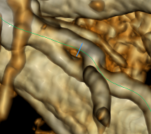
The figure below shows a three-dimensional reconstruction of the heart, obtained as a result of the work of a modern tomograph:

For the scale, the thickness of the aortic bulb is 3.2 cm, just think! However, when people have heart problems due to blood vessels, then, as a rule, we are not talking about such big ones. The image shows that the heart is surrounded by smaller vessels, and some of them branch directly from the large arteries. These are the so-called coronary arteries that feed the heart directly with blood. If narrowing of the lumen (stenosis) occurs in them, for example, due to the formation of calcium, then the blood flow decreases. When stenosis is pronounced, tissue necrosis occurs, in other words a heart attack. Next, I will talk about our approach to calculating the boundaries of blood vessels, which as a result allows you to automatically find the narrowing and give them an estimate.
To understand the material you need to have a superficial idea of the volume, voxels and their intensities. You can find out by reading the beginning of this article .
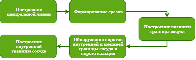
To evaluate the narrowing of a vessel, we need to know the lumen of the vessel or its internal border. To do this, you must at least detect all the calcium. We also find the outer boundary, because it makes it possible to estimate the wall thickness, which is also useful. To begin, let's take a look at the full border detection scheme, and then we will analyze each stage in detail:
Plotting the center line
The most difficult stage in terms of implementation (at least it took the most time). The method is based on the use of a Hessian matrix (Multi-Scale Vessel Segmentation Using Hessian Matrix Enhancement). More details in the already mentioned article .
Slicing
We only have a central line, and we need spatially dependent intensities of voxels that you can conveniently work with. To get them, a “stack” of slices is going. To begin with, fixed points are placed on the center line at fixed distances. Then a perpendicular is constructed from each point
 . After is the second perpendicular
  . Where
  is the direction of the center line at a point. Both perpendiculars are normalized. At each point of the
  center line of the vector
  form a 2d coordinate system. Thus, slices are formed:
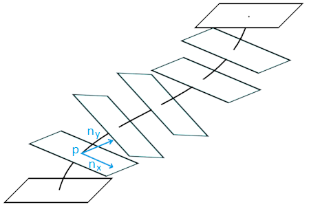
The voxel position is defined as
 , where
  , here
  are the real coordinates of the voxel, k is the slice number. Contact formula for the real coordinates
  . When moving to a new coordinate system, the space formed by the slices is simplified:
What we need!
Construction of the external border of the vessel
Let's take a look at the diagram:
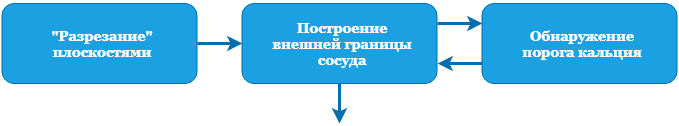
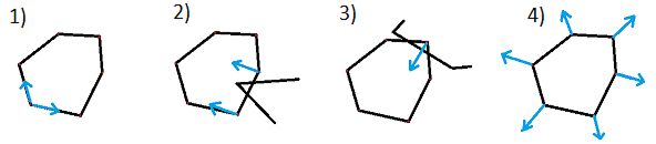
We cut our stack of slices obtained at the previous stage into eight planes (similar to cutting a cake) and we carry out all calculations in the space of planes:
Incision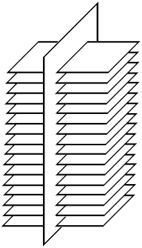
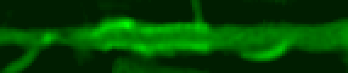
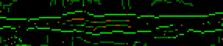
If you display the normalized values of the intensities of the voxels that hit the cutting plane, we get the following picture:
To detect the boundaries of the vessel, the classical approach (edge detection by gradient) is used in conjunction with the search for the path. Scheme:

1. Apply Gaussian smoothing with a small value
 to suppress noise:
 For a point with coordinates
 :,
:,  where
where  returns the value of intensity at a point
  ; r usually takes the value
  (
(  - rounding up); - smoothing coefficient.
 2. Each point is the gradient and its value, calculations are performed with smoothed intensity values:
 ,
, where
 - the partial derivatives. They are finite difference method:
  ,
, where
 - the intensity at the point after smoothing.
 Next, we need the direction of the gradient
 (
(  - normalization of the vector) and the value of the gradient
 (
(  Is the length of the vector)
 3. The direction of the gradient is translated into degrees or radians:
 (atan2 () is the arc tangent function in C ++, not to be confused with atan ()), then we round the angle so that it can have 4 values in increments of 45 degrees, t .e. top and bottom are considered the same direction:
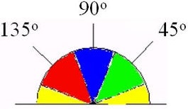
4. Perform suppression of non-maximums. If the gradient value
at least in one of two neighboring points (according to the direction of the gradient) is greater than or equal to the gradient value at the current point, then such a point cannot belong to the boundary: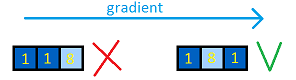
5. All remaining voxels are considered boundaries. Based on the value of the gradient, the threshold of calcium (which is not immediately available) and the proximity to the “vertical” center, each point is assigned a certain cost (the brighter the voxel, the higher its priority when searching for a path):
In this form, the boundaries of the vessel are already almost uniquely defined.
6, 7. To build boundaries, we use the search for the path. The closest extreme points with the least cost are taken as the initial and final. To search for a path, use a simple breadth-first search, which selects the least cost boundary points. Jumps are also available, but their price is high. The upper and lower boundaries of the vessel are searched separately, and then smoothing is applied to them:
Result
This procedure is performed for each plane, which results in sixteen-segment rings for each slice in the stack. These rings form the outer borders of the vessel.
As you can see from the image, there are areas in which the borders are detected incorrectly. This is due to the presence of calcium, which results in the detection of calcium boundaries rather than vessel boundaries. To prevent this from happening after the first detection of boundaries, it is necessary to determine the calcium threshold (more on this later), and then perform a second detection of boundaries, ignoring calcium-related voxels. Then we get:
Good result
After the external boundary is known, we need to collect statistical information. Namely, the intensities of all voxels that are inside the vessel.
Detection of thresholds of internal, external borders and calcium threshold
After the external boundary is known, we need to collect statistical information. Namely, the intensities of all voxels that are inside the vessel.
Threshold detection
Now consider the clustering algorithm expectation maximization (hereinafter referred to as EM). Let's start with the normal distribution function: it is characterized by the mathematical expectation
 and standard deviation . Here's how they affect the type of distribution:
Suppose we have data (points) that came from a “yellow” source and from a “blue” source:

Then, using standard formulas, we easily find the mean and standard deviation for each source. Formulas for source “a”:


But what if we know the number of sources, but don’t know which points belong to which source? What if we have such a picture?

If someone came and told us the distribution parameters, then we could easily calculate the probability of each point belonging to each of the sources. The probability that the point belongs to the source “a”:,
 where
where 

And if we need to calculate the source parameters, knowing the probabilities:


At start-up, EM receives some predefined parameters for sources, which can simply be selected randomly. Obviously, if the parameters are known, then we can calculate the probability of each point belonging to each of the sources. Now that the probabilities are known, we can calculate new more accurate parameters. Then it starts all over again, but with new parameters. After each cycle, the parameters of the sources are becoming more accurate.
How can we use this knowledge in relation to vessels? Let's take a look at the structure of one of them:
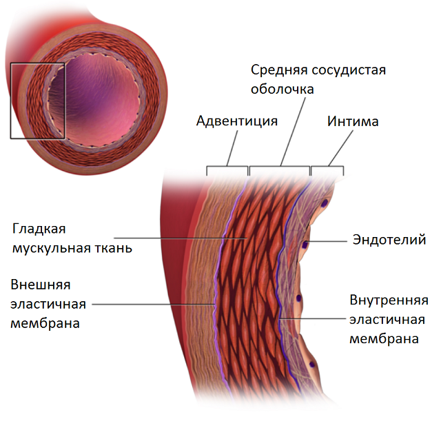
- fat
- wall # 1
- wall # 2
- contrast medium
- calcium
The distribution of voxel intensities in each case is normal. Those. we have everything we need to use EM to find the parameters of each source.
The results are good enough
The green line is a histogram of intensities, the red line is the resulting mathematical model.
The green line is a histogram of intensities, the red line is the resulting mathematical model.
Now that we know the parameters of each source, we can calculate the thresholds - the intensity values, at the intersection of which, the voxel membership changes from one source to another. We are interested in:
1. The threshold of the outer boundary of the vessel. If the voxel intensity is below this value, then it is considered that it does not belong to the vessel at all;
2. The threshold of the inner boundary of the vessel. If the voxel intensity is greater than this value, then it
refers to the lumen of the vessel, i.e. to a mixture of blood and contrast medium;
3. The threshold of calcium. If the value of the voxel intensity is greater than this value, then it refers to calcium.
Construction of the inner border of the vessel
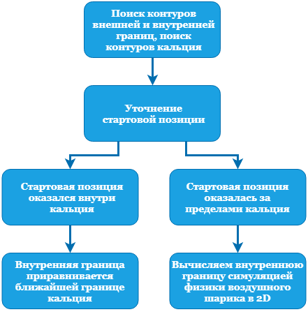
As always, let's start with the diagram; calculations are performed for each slice.
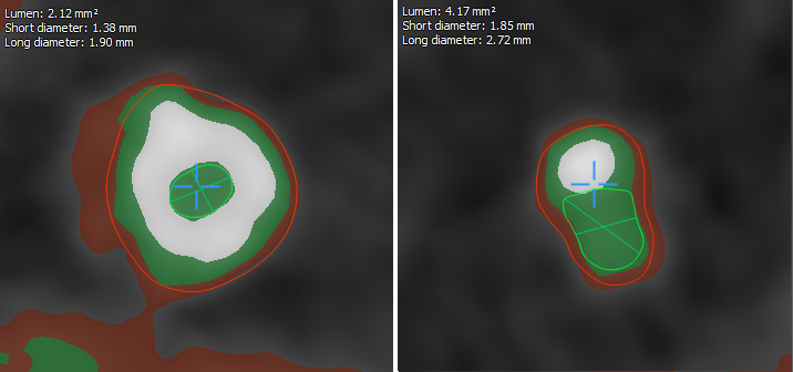
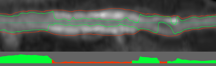
If you visually display the data according to the thresholds obtained in the previous step, we get the following picture:
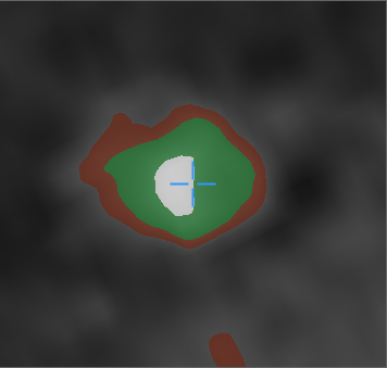
Red color is the wall of the vessel. Green color - clearance. White is calcium.
The first thing that catches your eye is the “hanging” calcium, which does not adjoin any of the walls. This is considered normal and occurs due to the smoothing applied by the tomograph itself.
First you need to get the boundaries according to the thresholds, and for this the marching squares algorithm is used. It can be said, passes in two stages. First, the area is divided by a discrete grid, and the squares in which the intensity values are greater than or equal to the threshold are considered “positive”, the rest are considered “negative”.

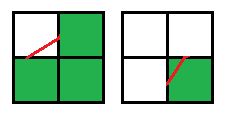
1. Three squares of one sign and one opposite, the movement of the contour occurs diagonally:
Example
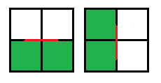
2. Two squares of the same sign and two opposite, and the squares with the same sign are located on one side, the movement of the contour is vertical or horizontal:
Example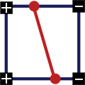
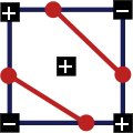
3. Two squares of the same sign and two opposite, squares with the same signs are placed on opposite sides:
Example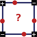
This is an exceptional case, in order to make a decision, the average value of intensity in all four squares is taken, and if it is greater than or equal to the threshold, then the center is positive, in other cases it is negative. It is also important which node is current at the moment:
Example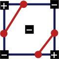
The marching squares algorithm accurately and unambiguously constructs a contour. In the example below, I deliberately shifted the line from the center of the side so that each step was clearly visible.
Example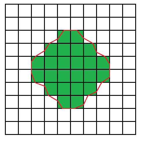 Specifically, the first and second cases:
For each section of the vessel, we find two main contours - this is the contour of the outer border and the contour of the inner border. We immediately “cut” the outer contour with our other outer contour, which we found at the beginning of the article by searching for paths. This is done to ignore the branches of the vessel. We ignore the contours of calcium that are too far from the inner wall, as if they do not exist at all, we find and use the rest in the future. If the center of the vessel is inside the calcium, then we shift it in the direction closest to the calcium circuit until the center is in the lumen (in the green region). Such an updated center, I will call the starting position.
According to the scheme, there can be two cases: simple and complex.
If the starting position is inside a closed calcium loop (for example, if a stent is installed), then we immediately equate the inner boundary to this loop. Things are more complicated when the center is outside of calcium. In this case, we need to expand the starting circuit so that it smoothly flows around calcium and the inner border:
To achieve the desired result, a special algorithm was developed based on ideas used in physical 2d engines, in particular polygons collisions solving and separate axis theorem.
Two basic concepts that can not be dispensed with: for intersecting convex polygons, the mtv vector (minimum translation vector) is the smallest displacement of one of the polygons, after which the intersection stops.


1. At each vertex of the starting contour, two forces act in the direction of neighboring vertices, and the forces are directly proportional to the distance to these vertices. This makes the outline shrink and strive to maintain a rounded shape;
2. If the vertex of the side contour falls inside the start contour, then the offset proportional to the vertex mtv vector of the vertex is applied to the nearest face of the start contour;
3. If the top of the start contour is inside the side contour, then the offset proportional to the vertex vector of the vertex is applied to the top of the start contour. This, together with the previous paragraph, does not allow the circuit to go beyond the boundaries of other circuits;
4. If cases 2 and 3 did not work for the vertex, then a force is applied to it in the averaged direction of the two normals of adjacent faces. This ensures the growth of the contour “in breadth”.
Thanks to this approach, we find the lumen of the vessel, taking into account the fact that calcium does not adjoin close to the walls. Now just combine the results from all sections and get the inner and outer borders of the vessel:
The apparent inaccuracy of the border after the stent is caused by anomalous bifurcation:
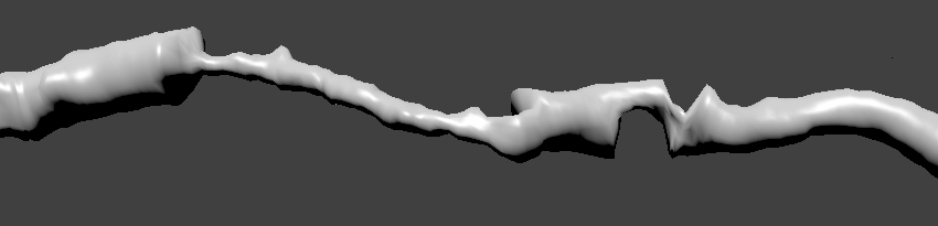
The area of the inner border at the cut will characterize the very clearance that we are ultimately interested in. Further use of this data I consider trivial and not requiring consideration. Finally, I’ll leave the image of the exported inner border in 3D: