How machines analyze big data: an introduction to clustering algorithms

Translation of How Machines Make Sense of Big Data: an Introduction to Clustering Algorithms .

Take a look at the picture below. This is a collection of insects (snails are not insects, but we will not find fault) of various shapes and sizes. Now divide them into several groups according to the degree of similarity. No catch. Start by grouping spiders.



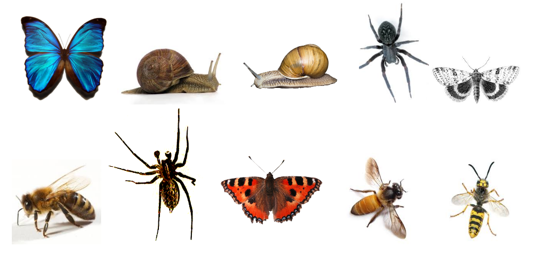
Finished? Although there is no “right” solution here, you must have divided these creatures into four clusters . In one cluster there are spiders, in the second - a pair of snails, in the third - butterflies, and in the fourth - a trio of bees and wasps.

Well done, right? You could probably do the same if there were twice as many insects in the picture. And if you had plenty of time - or a craving for entomology - then you probably would have grouped hundreds of insects.

However, for a machine, grouping ten objects into meaningful clusters is not an easy task. Thanks to such a complex branch of mathematics as combinatorics , we know that 10 insects are grouped in 115,975 ways. And if there are 20 insects, then the number of clustering options will exceed 50 trillion .

With a hundred insects, the number of possible solutions will be greater than the number of elementary particles in the known Universe . How much more? According to my estimates, approximatelyfive hundred million billion billion times more . It turns out more than four million billion google solutions ( what is google? ). And this is only for hundreds of objects.

Almost all of these combinations will be meaningless. Despite the unimaginable number of solutions, you yourself very quickly found one of the few useful ways of clustering.

We humans take for granted our excellent ability to catalog and understand large amounts of data. It does not matter whether it is text, or pictures on the screen, or a sequence of objects - people, in general, effectively understand the data coming from the surrounding world.

Given that a key aspect of AI development and machine learning is that machines can quickly understand large volumes of input data, how can I improve work efficiency? In this article, we will consider three clustering algorithms with which machines can quickly comprehend large amounts of data. This list is far from complete - there are other algorithms - but it is already quite possible to start with it.

For each algorithm, I will describe when it can be used, how it works, and I will also give an example with step-by-step analysis. I believe that for a real understanding of the algorithm, you need to repeat its work yourself. If you are really interested , you will realize that it is best to run algorithms on paper. Act, no one will blame you!


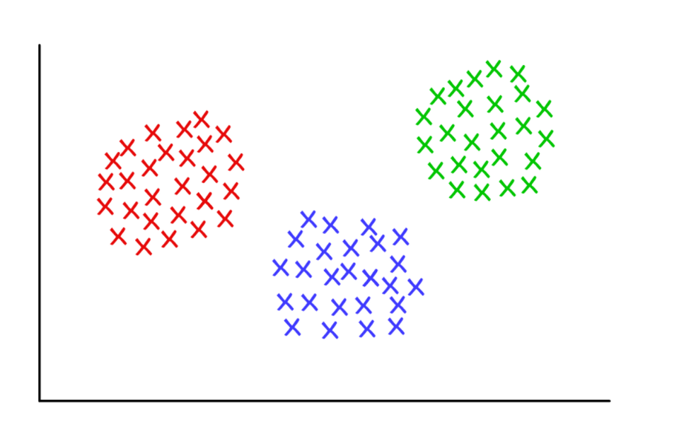
Three suspiciously neat clusters with k = 3

K-means clustering

Used by:

When you understand how many groups can be obtained to find a predetermined (a priori).

How does it work:

The algorithm randomly assigns each observation to one of k categories, and then calculates the average for each category. Then he reassigns each observation to the category with the nearest average, and again calculates the averages. The process is repeated until reassignments are needed.

Working example:

Take a group of 12 players and the number of goals scored by each of them in the current season (for example, in the range from 3 to 30). We divide the players, say, into three clusters.

Step 1 : you need to randomly divide the players into three groups and calculate the average for each of them.

Group 1
Player A (5 goals), Player B (20 goals), Player C (11 goals) 
Group Mean = (5 + 20 + 11) / 3 = 12
Group 2
Player D (5 goals), Player E (3 goals), Player F (19 goals)
Group Mean = 9
Group 3
Player G (30 goals), Player H (3 goals), Player I (15 goals)
Group Mean = 16

Step 2 : reassign each player to the group with the nearest average. For example, player A (5 goals) goes to group 2 (average = 9). Then again we calculate the group averages.

Group 1 (Old Mean = 12)
Player C (11 goals) 
New Mean = 11
Group 2 (Old Mean = 9)
Player A (5 goals), Player D (5 goals), Player E (3 goals), Player H (3 goals)
New Mean = 4
Group 3 (Old Mean = 16)
Player G (30 goals), Player I (15 goals), Player B (20 goals), Player F (19 goals)
New Mean = 21

Repeat step 2 again and again until the players stop changing groups. In this artificial example, this will happen at the next iteration. Stop! You have formed three clusters from a dataset!

Group 1 (Old Mean = 11)
Player C (11 goals), Player I (15 goals)
Final Mean = 13
Group 2 (Old Mean = 4)
Player A (5 goals), Player D (5 goals), Player E (3 goals), Player H (3 goals)
Final Mean = 4
Group 3 (Old Mean = 21)
Player G (30 goals), Player B (20 goals), Player F (19 goals)
Final Mean = 23

Clusters should correspond to the position of players on the field - defenders, central defenders and forwards. K-means work in this example because there is reason to believe that the data will be divided into these three categories.

Thus, based on the statistical variation in performance, the machine can justify the location of players on the field for any team sport. This is useful for sports analytics, as well as for any other tasks in which dividing the dataset into predefined groups helps to draw the appropriate conclusions.

There are several variations of the described algorithm. The initial formation of clusters can be performed in various ways. We examined the random classification of players into groups, followed by the calculation of averages. As a result, the initial group averages are close to each other, which increases repeatability.

An alternative approach is to form clusters consisting of only one player, and then group the players into the nearest clusters. The resulting clusters are more dependent on the initial stage of formation, and the repeatability in datasets with high variability decreases. But with this approach, it may take less iterations to complete the algorithm, because less time will be spent on splitting the groups.

The obvious drawback of k-means clustering is that you need to guess in advance how many clusters you have. There are methods for assessing the conformity of a particular set of clusters. For example, the intra- sum of the squares (Within-Cluster Sum-of- Squares) - a measure of the variability within each cluster. The “better” the clusters, the lower the total intracluster sum of squares.

Hierarchical clustering

Used by:

When you need to reveal the relationship between the values ​​(observations).

How does it work:

The distance matrix is ​​calculated in which the value of the cell ( i, j ) is the metric of the distance between the values ​​of i and j . Then a pair of the closest values ​​is taken and the average is calculated. A new distance matrix is ​​created, paired values ​​are combined into one object. Then a pair of the closest values ​​is taken from this new matrix and a new average value is calculated. The cycle repeats until all values ​​are grouped.

Working example:

Take an extremely simplified dataset with several species of whales and dolphins. I am a biologist, and I can assure you that much more properties are used to build phylogenetic trees . But for our example, we restrict ourselves to the characteristic body length of six species of marine mammals. There will be two stages of calculations.



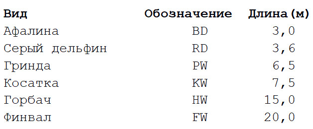
Step 1 : the matrix of distances between all views is calculated. We will use the Euclidean metric that describes how far our data is from each other, like the settlements on the map. You can get the difference in the length of the bodies of each pair by reading the value at the intersection of the corresponding column and row.



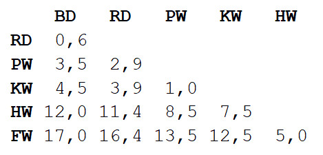
Step 2: A pair of two species closest to each other is taken. In this case, it is a bottlenose dolphin and a gray dolphin, whose average body length is 3.3 m.

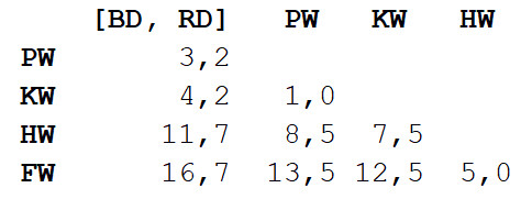
We repeat step 1, again calculating the distance matrix, but this time we combine bottlenose dolphin and gray dolphin into one object with a body length of 3.3 m.



Now we repeat step 2, but with a new distance matrix. This time, the grind and the killer whale will be the closest, so we will pair them and calculate the average - 7 m.

Next, repeat step 1: again, calculate the distance matrix, but with the grind and killer whale in the form of a single object with a body length of 7 m.



Repeat step 2 with this matrix. The smallest distance (3.7 m) will be between the two combined objects, so we will combine them into an even larger object and calculate the average value - 5.2 m.

Then repeat step 1 and calculate a new matrix by combining bottlenose dolphin / gray dolphin with grind / killer whale.



We repeat step 2. The smallest distance (5 m) will be between the humpback and the finwale, so we combine them and calculate the average - 17.5 m.

Again, step 1: we calculate the matrix.



Finally, repeat step 2 - there is only one distance left (12.3 m), so we will unite everyone into one object and stop. Here's what happened:

[[[BD, RD],[PW, KW]],[HW, FW]]

The object has a hierarchical structure (remember JSON ), so it can be displayed as a tree graph, or dendrogram. The result is similar to a family tree. The closer two values ​​are on a tree, the more they are similar or the more closely connected.


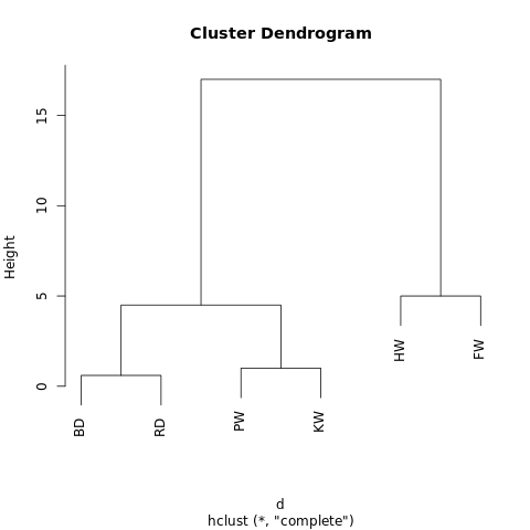
A simple dendrogram generated using R-Fiddle.org

The structure of the dendrogram allows you to understand the structure of the dataset itself. In our example, we got two main branches - one with a humpback and finwal, the other with a bottlenose dolphin / gray dolphin and a grind / killer whale.

In evolutionary biology, much larger datasets with many species and an abundance of characters are used to identify taxonomic relationships. Outside of biology, hierarchical clustering is applied in the areas of Data Mining and machine learning.

This approach does not require prediction of the required number of clusters. You can split the resulting dendrogram into clusters, “trimming” the tree at the desired height. You can choose the height in different ways, depending on the desired resolution of data clustering.
For example, if the above dendrogram is cut off at a height of 10, then we will intersect the two main branches, thereby dividing the dendrogram into two columns. If cut at a height of 2, then divide the dendrogram into three clusters.

Other hierarchical clustering algorithms may differ in three aspects from those described in this article.

The most important thing is the approach. Here we used agglomerative(agglomerative) method: start with individual values ​​and cyclically cluster them until you get one large cluster. An alternative (and computationally more complex) approach implies the reverse sequence: first one huge cluster is created, and then it is sequentially divided into ever smaller clusters until separate values ​​remain.

There are also several methods for calculating distance matrices. Euclidean metrics are sufficient for most tasks, but other metrics are better suited in some situations .

Finally, the merger criterion may vary.(linkage criterion). The relationship between clusters depends on their proximity to each other, but the definition of “proximity” can be different. In our example, we measured the distance between the average values ​​(or "centroids") of each group and combined the nearest groups in pairs. But you can use another definition.

Suppose each cluster consists of several discrete values. The distance between two clusters can be defined as the minimum (or maximum) distance between any of their values, as shown below. For different contexts, it is convenient to use different definitions of the join criterion.


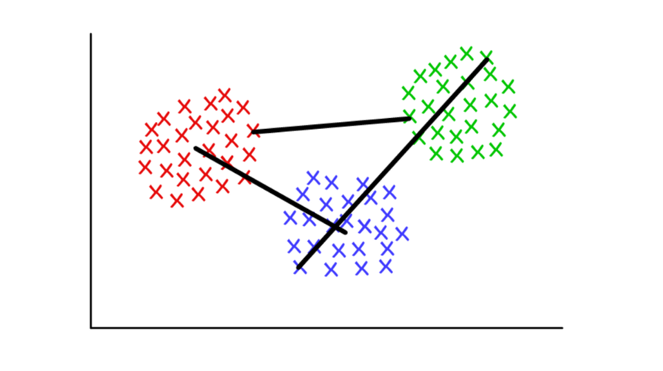
Red / blue: centroid pool; red / green: combining based on minima; green / blue: merging based on highs.

Definition of communities in graphs (Graph Community Detection)

Used by:

When your data can be presented in the form of a network, or "graph".

How does it work:

A community in a graph can be roughly defined as a subset of vertices that are more connected to each other than to the rest of the network. There are different community definition algorithms based on more specific definitions, such as Edge Betweenness, Modularity-Maximsation, Walktrap, Clique Percolation, Leading Eigenvector ...

Working example:

Graph theory is a very interesting section of mathematics that allows us to model complex systems in the form of abstract sets of “points” (vertices, nodes) connected by “lines” (edges).

Perhaps the first application of graphs that comes to mind is the study of social networks. In this case, the peaks represent people who are connected by ribs to friends / subscribers. But you can imagine any system in the form of a network if you can justify the method of meaningful connection of components. Innovative applications of clustering using graph theory include extracting properties from visual data and analyzing genetic regulatory networks.

As a simple example, let's look at the graph below. This shows the eight sites I visit most often. The links between them are based on links in Wikipedia articles. Such data can be collected manually, but for large projects it is much faster to write a Python script. For example, this: https://raw.githubusercontent.com/pg0408/Medium-articles/master/graph_maker.py .


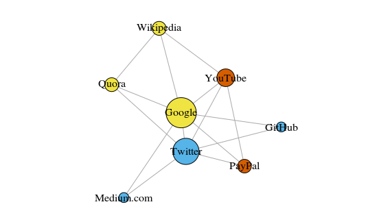
The graph is built using packet igraph for R 3.3.3

Color vertices depends on the participation in the community, and the size depends on the centrality (centrality). Please note that the most central are Google and Twitter.

Also, the resulting clusters very accurately reflect real tasks (this is always an important indicator of performance). The vertices representing the link / search sites are highlighted in yellow; blue highlighted sites for online publications (articles, tweets or code); highlighted in red are PayPal and YouTube, founded by former PayPal employees. Good deduction for the computer!

In addition to visualizing large systems, the true power of networks lies in mathematical analysis. Let's start by converting the network picture into a mathematical format. The following is the adjacency matrix of the network.



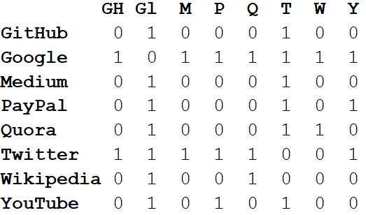
The values ​​at the intersections of columns and rows indicate whether there is an edge between this pair of vertices. For example, between Medium and Twitter it is, therefore, at the intersection of this line and the column there is 1. And between Medium and PayPal there is no edge, so in the corresponding cell there is 0.

If you represent all the network properties as an adjacency matrix, this will allow us to do all kinds useful findings. For example, the sum of the values ​​in any column or row characterizes the degree of each vertex - that is, the number of objects connected to this vertex. Usually indicated by the letter k .

If we sum the degrees of all the vertices and divide by two, we get L - the number of edges in the network. And the number of rows and columns is equal to N - the number of vertices in the network.

Knowing only k, L, N and the values ​​in all cells of the adjacency matrix A, we can calculate the modularity of any clustering.

Suppose we have clustered a network into a number of communities. Then you can use the modularity value to predict the “quality” of clustering. A higher modularity indicates that we divided the network into “exact” communities, and a lower modularity suggests that clusters are formed more by chance than reasonably. To make it clearer:


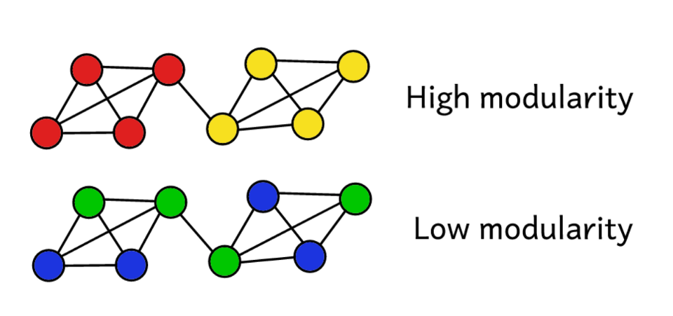
Modularity is a measure of the “quality” of groups.

Modularity can be calculated using the following formula:



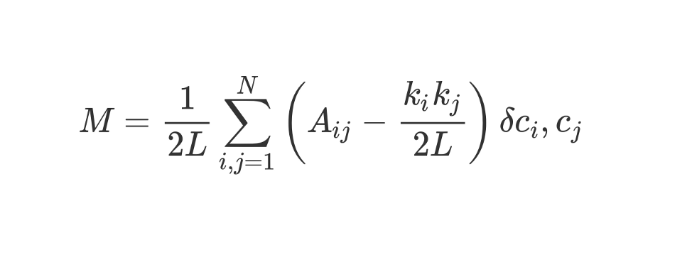
Let's look at this rather awesome looking formula.

M , as you know, this is modularity. 1 / 2L

ratiomeans that we divide the rest of the "body" of the formula by 2L, that is, by the double number of edges in the network. In Python, one could write:

sum = 0
for i in range(1,N):
    for j in range(1,N):
        ans = #stuff with i and j as indices
        sum += ans

What is it like #stuff with i and j? The bit in brackets tells us to subtract (k_i k_j) / 2L from A_ij, where A_ij is the value in the matrix at the intersection of row i and column j.

The values ​​k_i and k_j are the degrees of each vertex. They can be found by summing the values ​​in row i and column j, respectively. If we multiply them and divide by 2L, then we get the expected number of edges between the vertices i and j if the network were randomly mixed.

The contents of the brackets reflect the difference between the actual structure of the network and the expected one if the network were rebuilt randomly. If you play around with the values, then the highest modularity will be at A_ij = 1 and low (k_i k_j) / 2L. That is, modularity increases if there is an “unexpected” edge between the vertices i and j.

Finally, we multiply the contents of the brackets by what is indicated in the formula as δc_i, c_j. This is the Kronecker-delta function. Here is its implementation in Python:

def Kronecker_Delta(ci, cj):
    if ci == cj:
        return 1
    else:
        return 0
Kronecker_Delta("A","A")    #returns 1
Kronecker_Delta("A","B")    #returns 0

Yes, so simple. The function takes two arguments, and if they are identical, it returns 1, and if not, then 0.

In other words, if the vertices i and j fall into one cluster, then δc_i, c_j = 1. And if they are in different clusters, the function will return 0.

Since we multiply the contents of the brackets by the Kronecker symbol, the result of the invested sum Σ will be the highest when the vertices inside one cluster are joined by a large number of “unexpected” edges. Thus, modularity is an indicator of how well a graph is clustered into individual communities.

Division by 2L limits the upper modularity to unity. If the modularity is close to 0 or negative, this means that the current clustering of the network does not make sense. By increasing modularity, we can find a better way to cluster the network.

Please note that in order to evaluate the “quality” of clustering a graph, we need to determine in advance how it will be clustered. Unfortunately, unless the sample is very small, due to computational complexity it is simply physically impossible to stupidly go through all the methods of clustering a graph by comparing their modularity.

Combinatoricssuggests that for a network with 8 peaks, there are 4,140 clustering methods. For a network with 16 vertices, there will already be more than 10 billion ways, for a network with 32 vertices, 128 septillion, and for a network with 80 vertices, the number of clustering methods will exceed the number of atoms in the observable Universe .

Therefore, instead of enumeration, we will use the heuristic method, which will help to relatively easily calculate clusters with maximum modularity. This is an algorithm called Fast-Greedy Modularity-Maximization , a kind of analogue to the agglomerative hierarchical clustering algorithm described above. Instead of combining on the basis of proximity, Mod-Max unites communities depending on changes in modularity. How it works:

Firsteach vertex is assigned to its own community and the modularity of the entire network is calculated - M.

Step 1 : for each pair of communities connected by at least one edge, the algorithm calculates the resulting change in the modularity ΔM in the case of combining these pairs of communities.

Step 2 : then a pair is taken, when combined, ΔM will be maximum, and combined. For this clustering, a new modularity is calculated and stored.

Steps 1 and 2 are repeated : each time a pair of communities joins, which gives the largest ΔM, a new clustering scheme is saved, and its M.

Iterations stopwhen all the vertices are grouped into one huge cluster. Now the algorithm checks the stored records and finds the clustering scheme with the highest modularity. It is she who returns as a community structure.

It was computationally difficult, at least for people. Graph theory is a rich source of difficult computational problems and NP-hard problems. Using graphs, we can draw many useful conclusions about complex systems and datasets. Ask Larry Page, whose PageRank algorithm — which helped Google transform from a startup to a global dominant in less than a generation — is entirely based on graph theory.

Studies on graph theory today focus on identifying communities. There are many alternatives to the Modularity-Maximization algorithm, which, although useful, is not without its drawbacks.

First, with an agglomerative approach, small, well-defined communities are often combined into larger ones. This is called a resolution limit - the algorithm does not allocate communities smaller than a certain size. Another drawback is that instead of one pronounced, easily achievable global peak, the Mod-Max algorithm seeks to generate a wide "plateau" from many close modularity values. As a result, it is difficult to single out the winner.

Other algorithms use different methods for defining communities. For example, Edge-Betweenness is a divisive (dividing) algorithm that starts by grouping all the vertices into one huge cluster. Then the least “important” edges are iteratively removed until all vertices are isolated. The result is a hierarchical structure in which the vertices are closer to each other, the more they are similar.

The algorithm, Clique Percolation, takes into account possible intersections between communities. There is a group of algorithms based on random walk on a graph, and there are methods of spectral clustering, which deal with spectral decomposition (eigendecomposition) of the adjacency matrix and other matrices derived from it. All these ideas are used to highlight features, for example, in machine vision.

We will not analyze working examples for each algorithm in detail. Suffice it to say that today active research is being conducted in this direction and powerful data analysis techniques are being created, which it was extremely difficult to calculate 20 years ago.

Conclusion

I hope you learned something new for yourself, were able to better understand how, with the help of machine learning, you can analyze big data. The future is changing rapidly, and many changes will depend on what technology becomes available in the next 20-40 years.

As mentioned at the beginning, machine learning is an extremely ambitious field of research in which very complex tasks require the development of the most accurate and effective approaches. What is peculiar to people from nature, when transferred to a computer, requires innovative solutions.

The work is still endless, and those who propose the next breakthrough idea, no doubt, will be generously rewarded. Perhaps some of you readers will create a new powerful algorithm? All great ideas start somewhere!