Part 1. Introducing Marching cubes

How to create a mesh from any chaos
In Minecraft, we can dig in any direction, removing one block at a time with clearly defined edges. But in other games, developers are able to destroy the terrain smoothly, without cubic Minecraft.

Here is an example from No Man's Sky : video .

A similar technique is used to display images from MRI , metaballs and for voxelization of the relief.

In this part I will talk about the technique of creating a destructible relief Marching Cubes, and in a more general application - to create a smooth boundary mesh of a solid object. In this article, we will start by looking at two-dimensional techniques, then three-dimensional techniques, and in the third part we will look at Dual Contouring. Dual Contouring is a more advanced technique that creates the same effect.

Our goal

First, let's decide what we want to achieve. Suppose we have a function that can be discretized throughout the space, and we want to plot its boundary on the graph. In other words, determine where the function performs the transition from positive to negative and vice versa. In the example with a destructible relief, we will interpret the positive regions as solid and the negative regions as empty.

A function is a great way to describe an arbitrary shape. but she does not help us draw it.

To draw, we need to know its borderfor example, the points between positive and negative values, where the function intersects zero. The Marching Cubes algorithm takes such a function and creates a polygonal approximation of its border, which can be used for rendering. In 2d, this boundary will be a continuous line. When moving to 3d, it becomes a mesh.

The implementation of two-dimensional Marching Cubes

Note: this tutorial focuses more on concepts and ideas than implementation methods and code. If you are more interested in the implementation, then study the python code , which contains the commented code with everything you need.

For simplicity, let's start with 2d, and then move on to 3d. I will call the algorithms in 2d and 3d “Marching Cubes”, because in essence they are one algorithm.

Step 1

First, we divide the space into a uniform grid of squares (cells). Then, for each cell, by calculating the function, we can determine whether each vertex of the cell is inside or outside a solid region.

The function that describes the circle is shown below, and all the vertices whose coordinates are positive are marked with black dots.

Step 2

Then we process each cell separately, filling it with the corresponding border.


A simple lookup table provides 16 possible combinations of angles that are outside or inside. In each case, it determines which border should be drawn.


All combinations of two-dimensional marching cubes

Step 3

After repeating the process for all cells, the boundaries are joined, creating a ready mesh, even though each cell was considered independently.


Fine! I think this is generally similar to the original circle described by the formula. But as you can see, it is all broken, and the segments are located at angles of 45 degrees. It happened because we decided to select the vertices of the borders (red squares) equidistant from the points of the cell.

Adaptability

The best way to get rid of angles of 45 degrees is the adaptive marching cubes algorithm. Instead of simply specifying all the vertex boundaries from the central points of the cells, they can be positioned so that they best fit a solid area. To do this, we need not only to know whether the point is inside or outside; we also need to know how deep it is .

This means that we need some kind of function that gives us a measure of how deep the point is inside / outside. It does not have to be exact, because we use it only for approximations. In the case of our ideal circle having a radius of 2.5 units, we will use the following function .

$$f ( x , y ) = 2.5 - √x 2 + y 2

In which positive values ​​are inside, and negative values ​​are outside.

Then we can use numerical values$$f on either side of the face todetermine how far along the face you want the point to be.


If you put everything together, it will look like this:


Despite the fact that we have the same vertices and segments as before, a slight change in position makes the resulting figure much more like a circle.

Part 2. Three-dimensional Marching Cubes

So, in 2D, we divide the space into a grid, and then for each vertex of the cell we calculate where this point is located - inside or outside the solid region. In a 2d grid, each square has 4 angles, and for each of them there are two options, that is, each cell has$$2 × 2 × 2 × 2 = 2 4 = 16 possible combinations of angle states.

Then we fill the cell with our segment for each of 16 cases, and all segments of all cells naturally join together. We useadaptabilityto best fit these segments to the target surface.

The good newsis that in the three-dimensional case everything works almost the same. We divide the space into a grid of cubes, consider them separately, draw some edges for each cube, and they join together, creating the desired border mesh.

Bad news lies in the fact that the cube has 8 angles, that is, there $$2 8 = 256 cases considered. And some of these cases are much more complex than in 2D.

The very good newsis that we absolutely don't need to figure this out. You can simply copy thecases I have collectedand go straight to the section with the results (“Connecting everything together”), without thinking about all the difficulties. And then start reading about dual contouring if you need a more powerful technique.

All difficulties

Note: this tutorial focuses more on concepts and ideas than implementation methods and code. If you are more interested in the implementation, then study the implementation in 3D in python , which contains commented code with everything you need.

Are you still reading? Great, I like it.

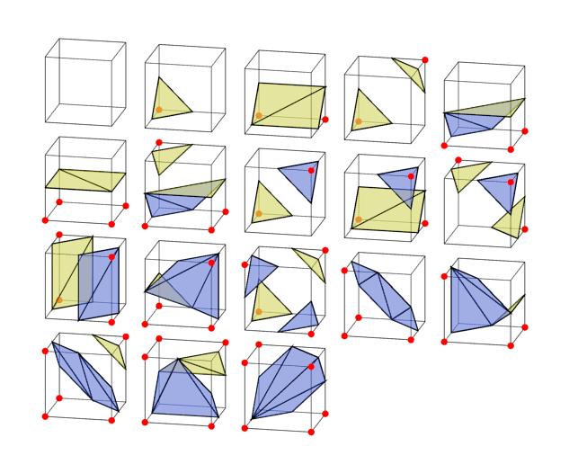
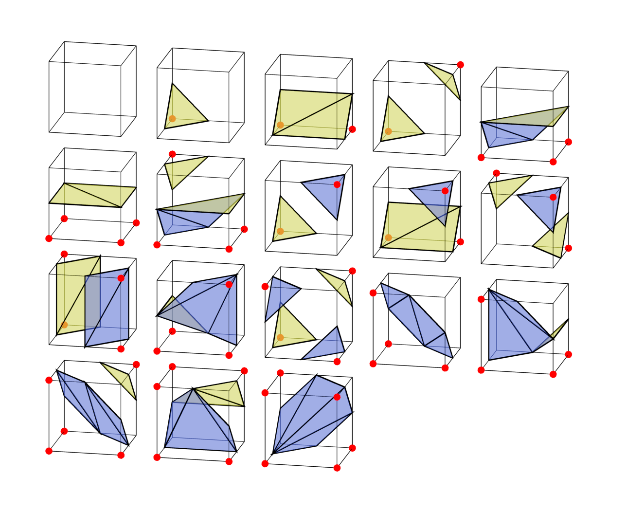
The secret is that we are not really required to collect all 256 different cases. Many of them are mirror images or turns of each other.


Here are three different cases of cells. Red corners are solid, all others are empty. In the first case, the lower corners are solid, and the upper ones are empty, therefore, to correctly draw the dividing border, it is necessary to divide the cell vertically. For convenience, I painted the outer side of the border yellow and the inside blue.

The remaining two cases can be found by simply turning the first case.

We can use one more trick:


These two cases are opposite to each other - the solid angles of one are empty of the other, and vice versa. We can easily generate one case from another - they have the same border, only turned upside down.

Given all this, in fact, we need to consider only 18 cases from which we can generate all the others.

Only intelligent person

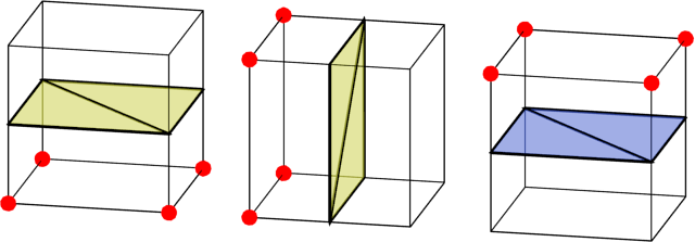
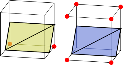
If you read the Wikipedia article or most of the Marching Cubes tutorials, they say that only 15 cases are needed. How so? Well, actually it's true - the three bottom cases from my circuit are not necessarily needed. Here again, these three cases in comparison with the other cases opposite them, giving a similar surface.


Both the second and third columns correctly separate solid angles from empty ones. But only when we consider one cube separately. If you look at the edges of each face of the cell, you can see that they differ for the second and third columns. Inverted will not properly connect to neighboring cells, leaving holes in the surface. After adding the extra three cases, all cells are connected correctly.

Putting it all together

As in the two-dimensional case, we can simply process all the cells independently. Here is a spherical mesh created from Marching Cubes.


As you can see, the shape of the sphere as a whole is done correctly, but in some parts there is chaos from narrow generated triangles. You can solve this problem using the Dual Contouring algorithm, which is more advanced than Marching Cubes.

Part 3. Dual Contouring

Marching Cubes are easy to implement, so they are often used. But the algorithm has many problems:

1. Complexity. Even though we only need to process one cube at a time, Marching Cubes as a result is quite complicated, because we need to consider many different cases.
   
   
   
2. Uncertainty. Some cases in Marching Cubes cannot obviously be resolved in one way or another. If in 2d we have two opposite angles, then it is impossible to say whether they should connect or not.
   
   
   
   
   In 3d, the problem is further compounded because an inconsistent election sequence can create a holey mesh. In the second part, we had to write additional code to solve this problem.
3. Marching Cubes cannot create sharp edges and corners. Here is a square approximated using Marching Cubes.
   
   
   
   
   The corners were cut. Adaptability cannot help here - Marching Squares always create straight lines inside any cell in which the corner of the target square appears.

What do we do?

Dual Contouring appears on the scene.

Note: this tutorial focuses more on concepts and ideas than implementation methods and code. If you are more interested in the implementation, then study the implementation in python, which contains commented code with everything you need ( 2d and 3d ).

Dual Contouring solves these problems and is much more extensible. Its disadvantage is that we need even more information about$$f ( x ) , that is, about the function that determines what is solid and empty. We need to know not only the meaning$$f ( x ) , but also the gradient$$f ′ ( x ) . This additional information will improve adaptability compared to marching cubes.

Dual Contouring places one vertex in each cell, and then “connects the dots”, creating a complete mesh. Points are connected along each edge that has a sign change, as in marching cubes.


Note: the word “dual” in the name appeared because the cells in the grid become the vertices of the mesh, which connects us with the dual graph .

Unlike Marching Cubes, we cannot calculate cells individually. To “connect the dots” and find the full mesh, we need to look at neighboring cells. But in fact, this is a much simpler algorithm than Marching Cubes, because there are not many individual cases. We simply find each edge with a change of sign and connect the vertices of the cells adjacent to this edge.

Getting a gradient

In our simple example with a 2d circle of radius 2.5 $$f is defined as follows:

$$f ( x , y ) = 2.5 - √x 2 + y 2

(in other words, 2.5 minus the distance from the center point)

Using the differential calculus, we can calculate the gradient:

$$f ′ ( x , y ) = Vec2 ( - x√x 2 + y 2 ,-y√x 2 + y 2 )

Gradient is a pair of numbers for each point, indicating how much the function changes when moving along the x or y axis.

But to obtain the gradient function, we do not need complex calculations. We can just measure change$$f when$$x and$$y deviate by a small amount$$d .

$$f ′ ( x , y ) ≈ Vec2 ( f ( x + d , y ) - f ( x - d , y )2 d ,f(x,y+d)-f(x,y-d)2 d )

It will work for any smooth $$f if selected$$d is small enough. In practice, it turns out that even functions with sharp points turn out to be quite smooth, because in order for this to work, it is not necessary to calculate the gradient next to sharp sections. Link to the code.

Adaptability

So far we have got the same stepped look that Marching Cubes had. We need to add adaptability. In the Marching Cubes algorithm, we chose where the vertex would be along the edge. Now we can freely select any point on the inside of the cell.

We want to choose the point that most closely matches the information we received, i.e. computed value

$$f ( x )

and gradient. Notice that we sampled the gradient along the edges, not at the corners.


Choosing the shown point, we guarantee that the displayed faces of this cell will correspond to the normals as much as possible:


In practice, not all normals in a cell will fit. We need to choose the most suitable point. In the last section I will tell you how to choose this point.

Go to 3d

The cases in 2d and 3d are not really very different. The cell is now a cube, not a square. We draw the edges, not the edges. But the differences end there. The procedure for selecting one point in a cell looks the same. And we still find the edges with a change of sign, and then we connect the points of the neighboring cells, but now there are already four cells, which gives us a four-sided polygon:


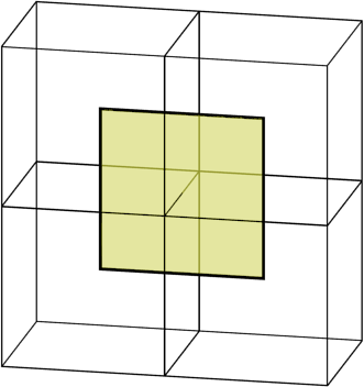
A face associated with a single edge. She has points in every neighboring cell.

results

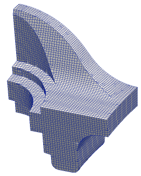
Dual contouring creates much more natural forms than marching cubes, which can be seen in the example of a sphere created with its help:


In 3d, this procedure is reliable enough to select points along the edge of a sharp section and to select angles when they occur.

Choosing a vertex location

A serious problem that I previously ignored is the location of the point in the case where the normals do not point to the same place.


In 3d, the problem is further exacerbated because there are more normals.

The solution is to select the point that is mutually best for all normals.

First, we assign a penalty to each normal for places far from ideal. Then we summarize all the penalty functions, which gives us a penalty in the form of an ellipse. After that, we select the point with the least penalty.


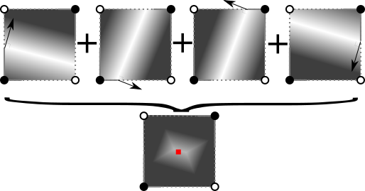
From a mathematical point of view, the individual penalty functions are the square of the distance from the ideal line for the current normal. The sum of all square terms is a quadratic function , so the common penalty function is called QEF (quadratic error function). Finding the minimum point of a quadratic function is a standard procedure that is available in most matrix libraries.

In my python implementation, I used the lstsq function from numpy.

Problems

Colinear normals

Most of the tutorials dwell on this, but the algorithm has a little dirty secret - the QEF solution as described in the original article on Dual Contouring does not really work very well.

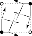
Having solved QEF, we can find the point that most closely matches the function normals. But in fact there is no guarantee that the resulting point is inside the cell .

In fact, quite often it is outside when we work with large flat surfaces. In this case, all sampled normals will be the same or very close, as in this figure.


I have seen many tips for solving this problem. Some people gave up, abandoning gradient information and using instead the center of the cell or the average of the border positions. This is called Surface Nets, and there is at least simplicity in that solution.

But based on my experience, I recommend using a combination of two techniques.

Technique 1: QEF Solution with Constraints

Do not forget that we found a cell point by finding a point that minimizes the value of a given function called QEF. After making small changes, we can find a minimizing point inside the cell.

Technique 2: QEF Offset

We can add any quadratic function to QEF and get another quadratic function, which will still be solvable. Therefore, I added a quadratic function that has a minimum point in the center of the cell.

Thanks to this, the whole QEF solution is pulled to the center.

In fact, this has a greater effect when the normals are collinear and most likely will give poor results, but have little effect on positions in a good case.

Using both techniques is pretty redundant, but it seems to me to give the best visual results.

Both techniques are shown in more detail in the code .

Self-intersections

Another dual contouring problem is that sometimes it can generate a self-intersecting 3d surface. In most cases, they do not pay attention to this, so I did not solve this problem.

There is an article that talks about her decision: “Intersection-free Contouring on An Octree Grid”, Ju and Udeshi, 2006

Uniformity

Although the resulting dual contouring mesh is always tight, the surface is not always well defined. Since there is only one point per cell, when two surfaces pass through the cell, it will be common to them. This is called a “homogeneous” mesh and can cause problems with some texturing algorithms. The problem often arises when solid objects are thinner than the size of a cell or several objects almost touch each other.


Handling such cases is a significant extension of the functionality of the basic Dual Contouring. If you need this feature, I recommend that you study this implementation of Dual Contouring or this article.

Algorithm Extension

Due to the relative simplicity of creating Dual Contouring meshes, it is much easier to extend to work with cell layouts that differ from the standard grids discussed above. Typically, an algorithm can be performed for octrees to get different cell sizes exactly where the details are needed. In general, the idea is similar - we select by a point per cell using sampled normals, then for each edge with a change of sign we find the neighboring 4 cells and combine their vertices into a face. In the octree, recursion can be used to find these edges and neighboring cells. Matt Keater has a detailed tutorial about this.

Another interesting extension is that for Dual Contouring we only need to determine what is inside / outside, and the corresponding normals. Although I said that we have a function for this, we can extract the same information from another mesh. This allows us to make a “strap”, i.e. generate a clean set of vertices and faces that clear the original mesh. An example is the remesh modifier from Blender.

Additional reading

• Adjacent Code
• Original article - Dual Contouring of Hermite Data - Tao Ju, Frank Losasso, Scott Schaefer, Joe Warren
• Dual Contouring is one of many similar techniques. See other approaches with their pros and cons in the SwiftCoder list .