Richard Hamming: Chapter 9. N-Dimensional Space

Hi, Habr. Remember the awesome article “You and Your Work” (+219, 2222 bookmarked, 350k reads)?

So Hamming (yes, yes, Hamming’s self-checking and self-correcting codes ) has a whole book written based on his lectures. We are translating it here, because the man is talking business.

This book is not just about IT, it is a book about the thinking style of incredibly cool people. “This is not just a charge of positive thinking; it describes conditions that increase the chances of doing a great job. ”

We have already translated 6 (out of 30) chapters.

Chapter 9. N-Dimensional Space

(Thanks for the translation, Alexei Fokin, who responded to my call in the "previous chapter.") Who wants to help with the translation - write in a personal email or magisterludi2016@yandex.ru

When I became a professor after 30 years of active research at Bell Telephone Laboratories, mainly in the department of mathematical research, I remembered that professors should reflect on and summarize past experience. I put my feet on the table and began to ponder my past. In the early years, I was mainly engaged in computing, that is, I was involved in many large projects requiring computing. Thinking about how several large engineering systems were developed, in which I was partially involved, I began, now at a certain distance from them, to see that they had many common elements. Over time, I began to realize that design tasks are in n-dimensional space, where n is the number of independent parameters. Yes, we create 3-dimensional objects, but their design is in a multidimensional space,

Multidimensional spaces will be needed so that further proofs become intuitive without rigorous detail. Therefore, we will now consider the n-dimensional space.

You think you live in three-dimensional space, but in many cases you live in two-dimensional space. For example, in a random course of life, if you meet someone, you have a reasonable chance of meeting this person again. But in the world of 3 dimensions there is no chance! Consider fish in the ocean that potentially live in three dimensions. They move along the surface or bottom, limiting things to two dimensions, or they form jambs, or gather in one place at the same time, such as a river mouth, beach, Sargasso sea, etc. They cannot expect to meet a buddy if they wander in the open ocean in three dimensions. Or, for example, if you want the planes to collide, you must collect them near the airport, place them in two-dimensional flight levels, or send them as a group;

N-dimensional space is a mathematical construct that we must explore in order to understand what happens to us when we roam there when solving design problems. In two dimensions, we have the Pythagorean theorem, for a right triangle the square of the hypotenuse is equal to the sum of the squares of the other sides. In three dimensions, we are interested in the length of the parallelepiped diagonal, Fig. 9.1. To find it, we first draw a diagonal of one face, apply the Pythagorean theorem, then take it as one of the sides with the other side of the third dimension, which is perpendicular to it, and again from the Pythagorean theorem we get that the square of the diagonal is the sum of the squares of three perpendicular sides. Obviously follows from this proof and the necessary symmetry of the formula,



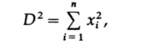
where x _{i are the} lengths of the sides of a rectangular block in n-dimensional space.


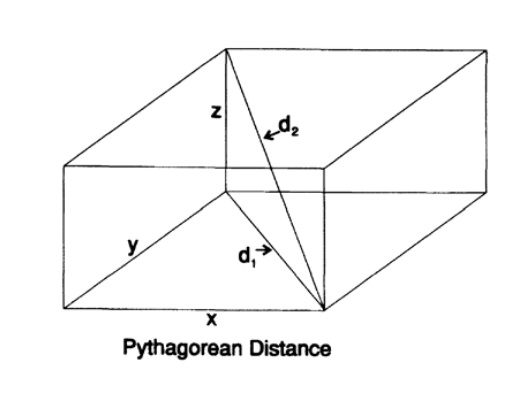
Fig. 9.I

Continuing the geometric approach, the planes in space will be just linear combinations of x _i , and the sphere around the point will be all points located at one fixed distance from the given one.

We need the volume of an n-dimensional sphere to understand the idea of ​​the size of a piece of limited space. But first, we need Stirling's approximation for n !, which I will bring out so that you understand most of the details and be sure of the correctness of what follows, and not take the word.

With a product of type n! difficult to handle, so we take log n !, which becomes



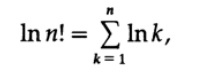
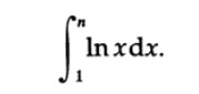
where, of course, ln is the base logarithm of e. The sums remind us that they are related to integrals, so we will start with such an integral



We apply integration by parts (since we know that ln x comes from the integration of an algebraic function and, therefore, can be excluded in the next step). Let U = ln x, dV = dx, then



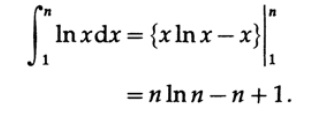
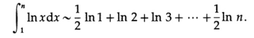
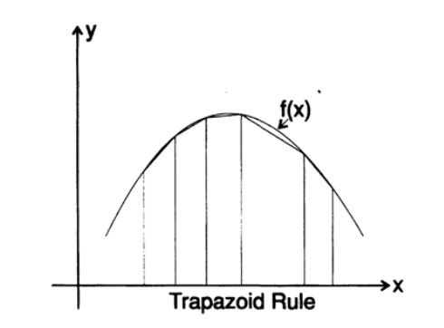
On the other hand, if we apply the trapezoid formula to the integral ln x we ​​get, see Fig. 9.II,



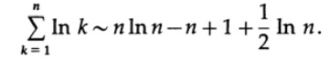
Since ln 1 = 0, adding (1/2) * ln n to both sides of the equality, we finally get



rid of the logarithms, raising e to the power of both sides.



where C is a certain constant (close to e), independent of n, since we approximated the integral with the trapezoid, the error grows more and more slowly and slowly with increasing n


. 9.II

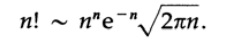
more and more, C has a limit. This is the first form of Stirling's formula. We will not waste time calculating the limit of the constant C while tending to infinity, which turns out to be √ (2 * π) = 2.5066 ... (e = 2.71828 ...). Thus, we finally obtain the Stirling formula for the factorial.



The following table shows the error of the Stirling approximation for n!



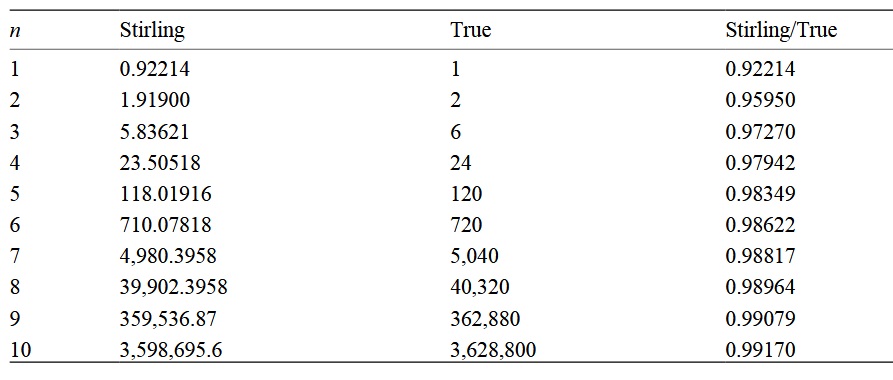
Please note that as the numbers increase, the coefficient approaches unity, but the difference becomes more and more!

If you consider 2 functions,



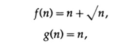
then the limit of the ratio f (n) / g (n) for n tending to infinity is 1, but as in the table, the difference



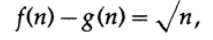
becomes more and more with increasing n.

We need to extend the concept of factorial to the set of all positive real numbers, for this we introduce a gamma function in the form of an integral



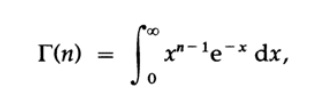
that exists for all n> 0. For n> 1, we again integrate by parts, this time using dV = e ^ (- x) dx and U = x ^ (n-1). For two limits, the integrable part is 0 and we have the following formula



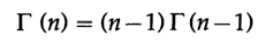
with Γ (1) = 1.

Thus, the gamma function takes values ​​(n-1)! for all positive integers n and naturally extends the concept of factorial to all positive numbers, since the integral exists for all n> 0.

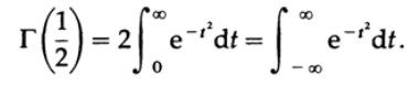
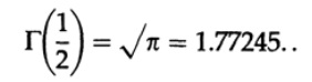
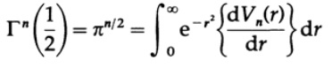
We need



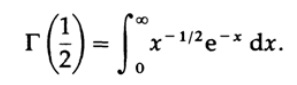
Denote x = t ^ 2, then dx = 2t * dt, and we obtain (using symmetry at the last step )



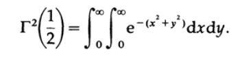
Now we use the standard approach to calculate this integral. We get the product of two integrals, one with respect to the variable x and one with respect to the variable y.



x ^ 2 + y ^ 2 imply polar coordinates, so we



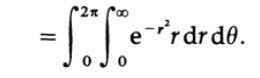
can easily convert angle integration. Exponential integration is now also easy, and we end up with.



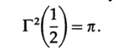
Thus,



now we return to the volume n of the dimensional sphere (or hyperspheres, if you want). It is clear that the volume of an n-dimensional cube with side x is x ^ n. After a little thought, you will realize that the formula for the volume of an n-dimensional sphere should have the form



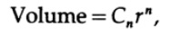
where C _{n is the} corresponding constant. For the case n = 2, the constant is π, for the case n = 1 it is 2 (if you think about it). In the three-dimensional case, we have C ₃= 4 * π / 3.

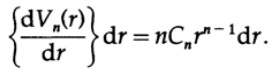
We start with the same trick that we used for gamma functions of 1/2, except this time we take the product of n integrals, each with its own variable x _i . The volume of the sphere can be represented as the sum of the volumes of the surfaces, each term of this sum corresponds to the surface area multiplied by the thickness dr. For a sphere, the value of the surface area can be obtained by differentiating the volume of the sphere with respect to the radius r,



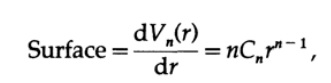
and therefore the terms of the volume are equal



Equating r ^ 2 = t, we




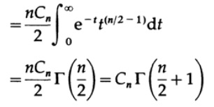
get where we get.



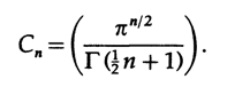
It is easy to see that



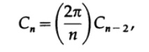
And we can calculate the following table.



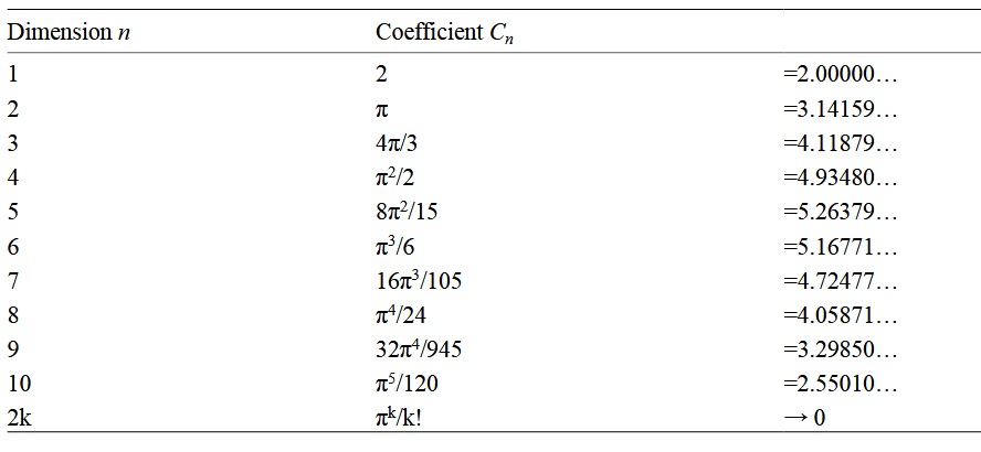
Thus, we see that the coefficient C _nincreases to n = 5, and then decreases to 0. For spheres of unit radius, this means that the volume of the sphere tends to zero with increasing dimension. If the radius is r, then for the volume, denoting n = 2k for convenience (since the real numbers change smoothly with increasing n and the spheres of odd dimensions are more difficult to calculate),


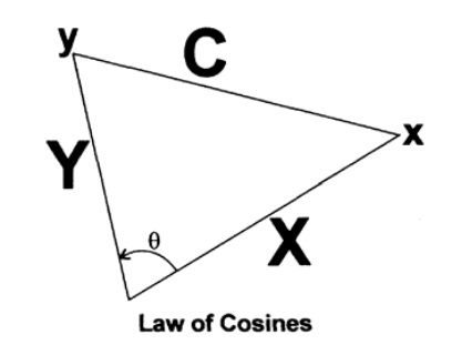
Fig. 9.III



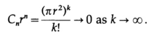
No matter how large the radius r, an increase in the number of measurements n gives rise to a sphere of arbitrarily small volume.

Now consider the relative amount of volume located close to the surface of the n-dimensional sphere. Let r be the radius of the sphere and the inner radius of the surface r (1-ε), then the relative volume of the surface is



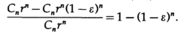
For large n, no matter how thin (in relation to the radius) the surface inside it is almost nothing. As we say, the volume is almost all on the surface. Even in 3 dimensional space, a single sphere has 7/8 of the volume inside the surface with a thickness of 1/2 radius. In n-dimensional space, 1- (1/2) ^ n is inside half the radius of the surface.

This is important in design; It turns out after calculations and data transformations above that almost certainly the optimal design will be on the surface, and not deep inside as you might think. Computational methods are usually not suitable for finding the optimum in multidimensional spaces. This is not at all strange; generally speaking, the best design is to bring one or more parameters to its extreme - it is obvious that you will find yourself on the surface of the visible area of ​​the design!

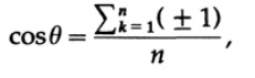
Next, we consider the diagonal of an n-dimensional cube, in other words, the vector from the origin to the point with coordinates (1,1, ..., 1). The cosine of the angle between this line and any axis is given by definition as the ratio of the value of the coordinate of the length of the projection onto this axis, which is obviously equal to 1 to the length of the vector, which is √n. Therefore,



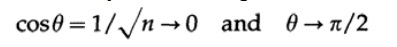
it follows that for large n the diagonal is almost perpendicular to each coordinate axis!

If we consider points with coordinates (± 1, ± 1, ..., ± 1) then there will be 2n diagonals such that all are almost perpendicular to each coordinate axis. For n = 10, for example, their number is 1024 such almost perpendicular lines.

I need an angle between two vectors, and although you may remember that this is a scalar product of vectors, I suggest that you print it again to better understand what is happening. [Remark; I found it very useful in important situations to revise all the basic involved inferences in order to feel what is happening.] Take two points x and y, with the corresponding coordinates x _i and y _i . Fig. 9.III. Applying the cosine theorem in the plane of 3 points x, y and the origin, we have



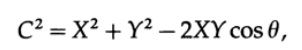
where X and Y are the lengths of the segments to the points x and y. But C can be obtained using the difference of coordinates on each axis.



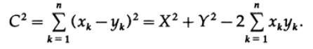
Equating the two expressions we see.



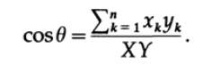
Now we apply this formula for two segments drawn from the origin to a random point from the coordinate set

(± 1, ± 1, ..., ± 1)

The scalar product of two such factors, taken at random, is again ± 1 and this should be summed n times, with the length of each segment being √n, therefore (note n in the denominator )



and by the weak law of large numbers this tends to 0 with an increase in n almost surely. But there are 2 ^ n random vectors and for a given vector, all the rest of the 2 ^ n random vectors are almost certainly almost perpendicular to this one! n-dimensionality is really vast!

In linear algebra and other disciplines, you have learned to find many perpendicular axes and then represent everything else in this coordinate system, but you see that in n-dimensional space after you find n mutually perpendicular coordinate axes, there are 2 ^ n other directions almost perpendicular to the ones you found! The theory and practice of linear algebra are completely different!

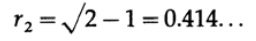
Finally, for further proof that your intuition about n-dimensional space is not very good, I will produce another paradox that I will need in the following chapters. We start with a 4x4 square divided by 4 unit squares, in each of which we draw a unit circle, Fig. 9.IV. Next, we draw a circle centered in the center of the square, touching the rest from the inside. Its radius should be from Fig. 9.IV,



In 3-dimensional space we have a 4x4x4 cube and 8 spheres of unit radius. The inner sphere touching the rest at a point lying on the segments connecting the centers has a radius.



Think about why its radius is greater than for 2 measurements.

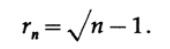
Moving to n dimensions, we have a 4x4x ... x4 cube and 2 ^ n spheres, one in each corner, each touching the remaining n neighboring ones. The inner sphere, touching the inside of the rest, will have a radius.



Check this carefully! You are sure? If not, why not? Where is the mistake in reasoning?
Having made sure that this is true, it is applicable for the case of n = 10 measurements. For the inner sphere, we have a radius of





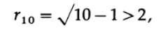
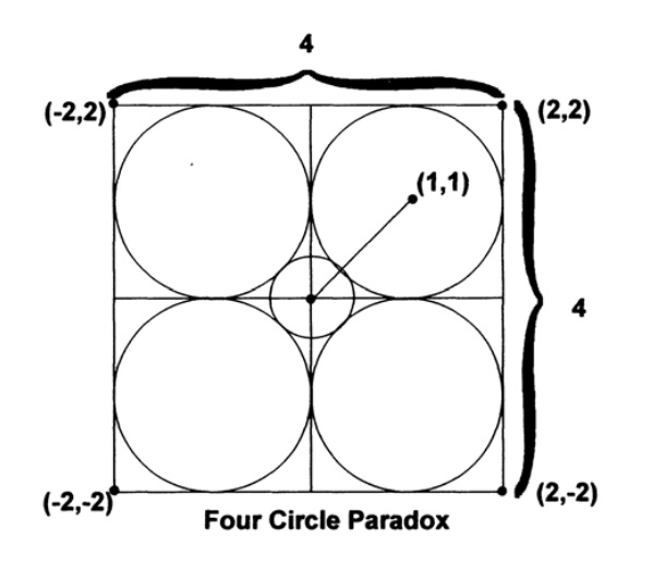
Fig. 9.IV

and in 10 dimensional space, the inner sphere went beyond the cube. Yes, the sphere is convex, yes, it touches the remaining 1024 from the inside, and at the same time it goes beyond the cube!

This is too much for your sensitive intuition about n-dimensional space, but remember that n-dimensional space is the place where complex objects are usually designed. You should try to better feel the n-dimensional space, thinking about the things just described, until you start to see how they can be true, or rather why they should be true. Otherwise, you will have problems when you will solve the complex design problem. Perhaps you should re-calculate the radii of different dimensions, as well as return to the angles between the diagonals and the coordinate axes and see how it turns out.

Now it must be strictly noted that I did all this in the classical Euclidean space using the Pythagorean distance, where the sum of the squares of the differences of the corresponding coordinates is equal to the square of the distance between the points. Mathematicians call this distance L ₂ .

Space L ₁It doesn’t use the sum of the squares of the coordinate differences, but rather the sum of the distances, as if you are traveling around a city with a rectangular street grid. This is the sum of the differences between the two points, which tells you how far you will have to go. In the computing industry, this is often referred to as the “Hamming distance” for reasons that will become clear in later chapters. In this space, a circle in two dimensions looks like a square standing on top, Fig. 9.V. In three-dimensional space, it’s like a cube standing on top, etc. Now you can better see how the paradoxical inner sphere from the above example can go beyond the cube.

There is a third, often used, metric (all of them are metrics = distance functions) called L _∞, or Chebyshev distance. Here, the maximum coordinate difference is taken for the distance, regardless of other differences, Fig. 9.VI. In this space, a circle is a square, a 3-dimensional sphere is a cube, and you see that in this case the inner sphere from the paradox has a zero radius in all directions.

These were examples of metrics, measures of distance. The conditions for determining the metric D (x, y) between two points x and y are as follows:

1. D (x, y) ≥ 0 (non-negative)
2. D (x, y) = 0 if and only if x = y ( identity)
3. D (x, y) = D (y, x) (symmetry)
4. D (x, y) + D (y, z) ≥ D (x, z) (triangle inequality).



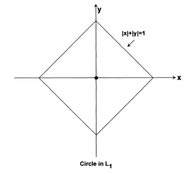
Fig. 9.V



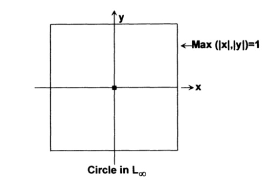
Fig. 9. VI

I leave you to check that the three metrics L _∞ , L ₂ and L ₁(Chebyshev, Pythagoras and Hamming) all satisfy these conditions.

The truth is that in complex design for various coordinates, we can use any of these metrics mixed together, so the design space is not a complete picture, but a mixture of pieces and parts. The L ₂ metric is obviously connected with the least squares, and the other two L _∞ and L _{1 are} more similar to comparisons. In comparisons in real life, you usually use either the maximum difference L _∞ in any one characteristic as a sufficient condition for distinguishing between two objects, or sometimes, as in a string of bits, this is the number of mismatches, which is significant, and the sum of squares does not fit, which means what is used L ₁metrics. This is more true for identifying patterns in AI.

Unfortunately, although everything described above is true, it is rarely revealed to you. No one ever told me that! I will need a lot of the results in the subsequent chapters, but generally speaking after this demonstration you should be better prepared than before for complex design and for a thorough analysis of the space in which the design is carried out, as I tried to do. The mess is basically where the design comes in, and you have to find an acceptable solution.

Since L ₁ and L _{∞ are} not well known, let me make a few remarks on the three metrics. L ₂a natural distance function for use in physical and geometric cases, including extracting data from physical measurements. Therefore, in physics you will find L ₂ everywhere . But when it comes to intellectual judgment, the other 2 metrics are more suitable, although this is slowly perceived, so we often see frequent use of the chi-square estimate, which is obviously a measure of L ₂ , where other more suitable estimates should be used.

To be continued ...

Who wants to help with the translation - write in a personal email or e-mail magisterludi2016@yandex.ru