Integration of equations of motion

A simulation of physics makes small predictions based on the laws of physics. These predictions are actually quite simple, something like "if an object is here and it moves at such a speed in this direction, then in a short period of time it will be here." We create such predictions using a mathematical technique called integration.

The topic of this article will be exactly the implementation of such integration.

Integration of equations of motion

You can remember from a course at a high school or university that force is equal to the product of mass and acceleration.

$$

We transform this equation and see that the acceleration is equal to the force divided by the mass. This is in line with our intuitive expectations, because heavy objects are harder to throw.

$$

Acceleration is the rate of change of speed over time:

$$

Similarly, speed is the rate at which a position changes over time:

$$

This means that if we know the current position and speed of the object, as well as the forces applied to it, we can integrate to find its position and speed at a certain point in time.

Numerical integration

If you have not studied differential equations at a university, you can breathe easy - you are almost in the same situation as those who studied them, because we will not solve differential equations analytically. Instead, we will seek a solution by numerical integration .

Here's how numerical integration works: first, start with the starting position and speed, then take a small step forward to find the speed and position in the future. Then we repeat this, moving forward in small steps, using the result of previous calculations as the starting point of the next.

But how do we find a change in speed and position at every step?

The answer lies in the equations of motion .

Let's call our current time t, and the time step is dt or “delta time”.

Now we can represent the equations of motion in an understandable way:

    acceleration = force / mass
    change of position = speed * dt
    speed change = acceleration * dt

Intuitively, this is understandable: if you are in a car moving at a speed of 60 km / h, then in one hour you will drive 60 km. Similarly, a car accelerating at 10 km / h per second will move 100 km / h faster in 10 seconds.

Of course, this logic is preserved only when the acceleration and speed are constant. But even if they change, this is a good approximation for a start.

Let's imagine this in code. We start with a stationary object weighing one kilogram and apply a constant force of 10 kN (kilonewtons) to it and take a step forward, assuming that one time step is equal to one second:

    double t = 0.0;
    float dt = 1.0f;
    float velocity = 0.0f;
    float position = 0.0f;
    float force = 10.0f;
    float mass = 1.0f;
    while ( t <= 10.0 )
    {
        position = position + velocity * dt;
        velocity = velocity + ( force / mass ) * dt;
        t += dt;
    }

Here is the result:

    t=0:    position = 0      velocity = 0
    t=1:    position = 0      velocity = 10
    t=2:    position = 10     velocity = 20
    t=3:    position = 30     velocity = 30
    t=4:    position = 60     velocity = 40
    t=5:    position = 100    velocity = 50
    t=6:    position = 150    velocity = 60
    t=7:    position = 210    velocity = 70
    t=8:    position = 280    velocity = 80
    t=9:    position = 360    velocity = 90
    t=10:   position = 450    velocity = 100

As you can see, at every step we know both the position and speed of the object. This is numerical integration.

Explicit Euler Method

The kind of integration we just used is called the explicit Euler method .

It is named after the Swiss mathematician Leonard Euler , who first discovered this technique.

Euler integration is the simplest technique of numerical integration. It is 100% accurate only when the rate of change over a time step is constant.

Since the acceleration in the example above is constant, speed integration is error-free. However, we also integrate speed to obtain a position, and speed increases due to acceleration. This means that an error occurs in the integrated position.

But how big is this mistake? Let's find out!

There is an analytical solution to the movement of an object with constant acceleration. We can use it to compare the numerically integrated position with the exact result:

    s = ut + 0.5at ^ 2
    s = 0.0 * t + 0.5at ^ 2
    s = 0.5 (10) (10 ^ 2)
    s = 0.5 (10) (100)
    s = 500 meters

After 10 seconds, the object was supposed to move 500 meters, but explicitly the Euler method gives us a result of 450. That is, an error of as much as 50 meters in just 10 seconds!

It seems that this is incredibly bad, but in games usually not such a large time interval is taken for the physics step. In fact, physics is usually calculated at a frequency approximately equal to the frame rate of the display.

If you set the step dt = ¹ ⁄ ₁₀₀ , then we will get a much better result:

    t=9.90:     position = 489.552155     velocity = 98.999062
    t=9.91:     position = 490.542145     velocity = 99.099060
    t=9.92:     position = 491.533142     velocity = 99.199059
    t=9.93:     position = 492.525146     velocity = 99.299057
    t=9.94:     position = 493.518127     velocity = 99.399055
    t=9.95:     position = 494.512115     velocity = 99.499054
    t=9.96:     position = 495.507111     velocity = 99.599052
    t=9.97:     position = 496.503113     velocity = 99.699051
    t=9.98:     position = 497.500092     velocity = 99.799049
    t=9.99:     position = 498.498077     velocity = 99.899048
    t=10.00:    position = 499.497070     velocity = 99.999046

As you can see, this is a pretty good result, definitely quite enough for the game.

Why Euler's explicit method is not (always) so good

With a sufficiently small time step, the explicit Euler method with constant acceleration gives quite decent results, but what happens if the acceleration is not constant?

A good example of variable acceleration is the spring shock absorber system .

In this system, the mass is attached to the spring, and its motion is suppressed by something like friction. There is a force proportional to the distance to the object, which draws it to the starting point, and a force proportional to the speed of the object, but directed in the opposite direction, which slows it down.

Here, the acceleration during the time step exactly changes, but this constantly changing function is a combination of position and speed, which themselves constantly change during the time step.

Here is an exampleharmonic oscillator with attenuation . This is a well-studied problem, and for it there is an analytical solution that can be used to verify the result of numerical integration.

Let's start with a weakly damped system, in which the mass oscillates near the starting point, gradually slowing down.

Here are the input parameters of the mass-spring system:

• Weight: 1 kilogram
• Starting position: 1000 meters from the starting point
• Hooke's coefficient of elasticity: k = 15
• Hooke law attenuation coefficient: b = 0.1

And here is a graph of the exact solution:



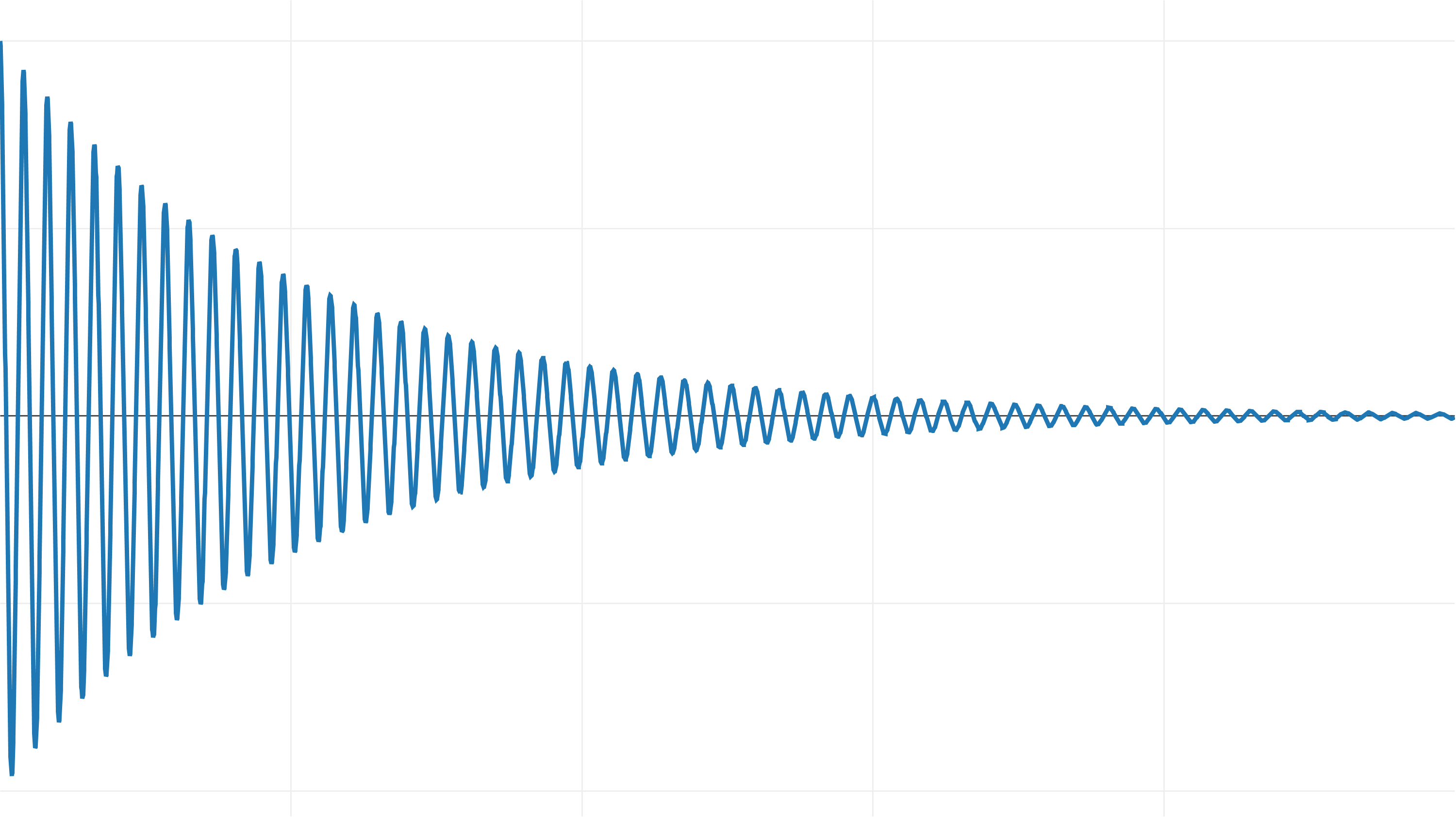
If we use the explicit Euler method to integrate this system, we get the following result, which I scaled vertically:



Instead of attenuation and approaching the starting point, the system gains energy over time!

When integrating explicitly by Euler and with dt = ¹ ⁄ _100, such a system is unstable.

Unfortunately, since we already integrate with a small time step, we do not have practical ways to improve accuracy. Even if we reduce the time step, there will always be an elastic coefficient k at which we obtain this behavior.

The symplectic Euler method

We can consider another integrator - the symplectic Euler method .

Most commercial game physics engines use this integrator.

The transition from the explicit to the symplectic Euler method consists only in replacing:

    position += velocity * dt;
    velocity += acceleration * dt;

on the:

    velocity += acceleration * dt;
    position += velocity * dt;

Using the symplectic Euler integrator for dt = ¹ ⁄ ₁₀₀ for a spring shock absorber system gives a stable result, very close to the exact solution:



Even though the symplectic Euler method has the same degree of accuracy as the explicit method (degree 1), when integrating the equations of motion, we get a much better result, because it is symplectic .

There are many other integration methods.

And now something is completely different.

The implicit Euler method is an integration method that is well suited for integrating stiff equations that become unstable with other methods. Its disadvantage is that it requires solving a system of equations at each time step.

Verlet integration provides greater accuracy than the implicit Euler method and requires less memory when simulating a large number of particles. This is an integrator of the second degree, which is also symplectic.

There is a whole family of integrators called Runge-Kutta methods. In fact, the explicit Euler method is considered part of this family, but it also includes integrators of a higher order, the most classic of which is the Runge-Kutta order 4 method or just RK4 .

This family of integrators is named after the German physicists who discovered them: Karl Runge and Martin Kutta .

RK4 is a fourth-order integrator, that is, the accumulated error is of the fourth-derivative order. This makes the method very accurate, much more accurate than the explicit and implicit Euler methods, which have only the first order.

But although it is more accurate, it cannot be said that RK4 automatically becomes the “best” integrator, or even that it is better than the symplectic Euler method. Everything is much more complicated. Nevertheless, it is a rather interesting integrator and is worth exploring.

RK4 implementation

There are already many explanations for the math used in RK4. For example: here , here and here . I highly recommend studying its derivation and understanding how and why it works at the mathematical level. But I understand that the target audience of this article is programmers, not mathematicians, so we will only consider implementation here. So let's get started.

Before we get started, let's set the state of the object as a struct in C ++ so that you can conveniently store position and speed in one place:

    struct State
    {
        float x;      // позиция
        float v;      // скорость
    };

We also need a structure for storing derived state values:

    struct Derivative
    {
        float dx;      // dx/dt = скорость
        float dv;      // dv/dt = ускорение
    };

Now we need a function to calculate the state of physics from t to t + dt using one set of derivatives, and then to calculate the derivatives in the new state:

    Derivative evaluate( const State & initial, 
                         double t, 
                         float dt, 
                         const Derivative & d )
    {
        State state;
        state.x = initial.x + d.dx*dt;
        state.v = initial.v + d.dv*dt;
        Derivative output;
        output.dx = state.v;
        output.dv = acceleration( state, t+dt );
        return output;
    }

The acceleration function controls the entire simulation. Let's use it in a spring shock absorber system and return the acceleration for a unit mass:

    float acceleration( const State & state, double t )
    {
        const float k = 15.0f;
        const float b = 0.1f;
        return -k * state.x - b * state.v;
    }

What you need to write here, of course, depends on the simulation, but you need to structure the simulation in such a way that it is possible to calculate the acceleration inside this method for the given state and time, otherwise it will not work for the RK4 integrator.

Finally, we get the integration procedure itself:

    void integrate( State & state, 
                    double t, 
                    float dt )
    {
        Derivative a,b,c,d;
        a = evaluate( state, t, 0.0f, Derivative() );
        b = evaluate( state, t, dt*0.5f, a );
        c = evaluate( state, t, dt*0.5f, b );
        d = evaluate( state, t, dt, c );
        float dxdt = 1.0f / 6.0f * 
            ( a.dx + 2.0f * ( b.dx + c.dx ) + d.dx );
        float dvdt = 1.0f / 6.0f * 
            ( a.dv + 2.0f * ( b.dv + c.dv ) + d.dv );
        state.x = state.x + dxdt * dt;
        state.v = state.v + dvdt * dt;
    }

The RK4 integrator samples the derivative at four points to determine the curvature. Notice how the derivative a is used in the calculation of b, b is used in the calculation of c, and c for d. This transfer of the current derivative to the calculation of the next gives the integrator RK4 its accuracy.

It is important that each of these derivatives a, b, c and d will be different when the rate of change in these quantities is a function of time or a function of the state itself. For example, in our spring shock absorber system, acceleration is a function of the current position and speed, which vary in time step.

After calculating the four derivatives, the best total derivative is calculated as the weighted sum obtained from the expansion in the Taylor series. This combined derivative is used to move position and speed forward in time, just like we did in the explicit Euler integrator.

Comparison of the symplectic Euler method and RK4

Let's test the integrator RK4.

Obviously, since it is a higher-order integrator (fourth versus first), it will clearly be more accurate than the Euler symplectic method, right?



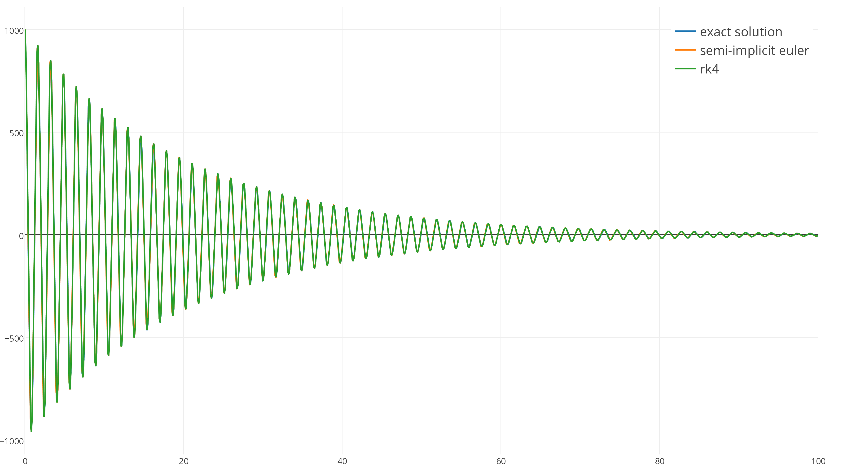
Not true . Both integrators are so close to the exact result that at this scale it is almost impossible to find the difference between them. Both integrators are stable and repeat the exact solution very well at dt = ¹ ⁄ ₁₀₀ .


With an increase, it is clear that RK4 is indeed more accurate than the symplectic Euler method, but is this accuracy worth the complexity and extra execution time of RK4? Hard to judge.

Let's try and see if we can find a significant difference between the two integrators. Unfortunately, we will not be able to observe this system for a long time, because it quickly fades to zero, so let's move on to a simple harmonic oscillator that oscillates endlessly and without attenuation.

Here is the exact result that we will strive for:



To complicate the task for integrators, let's increase the time step to 0.1 seconds.

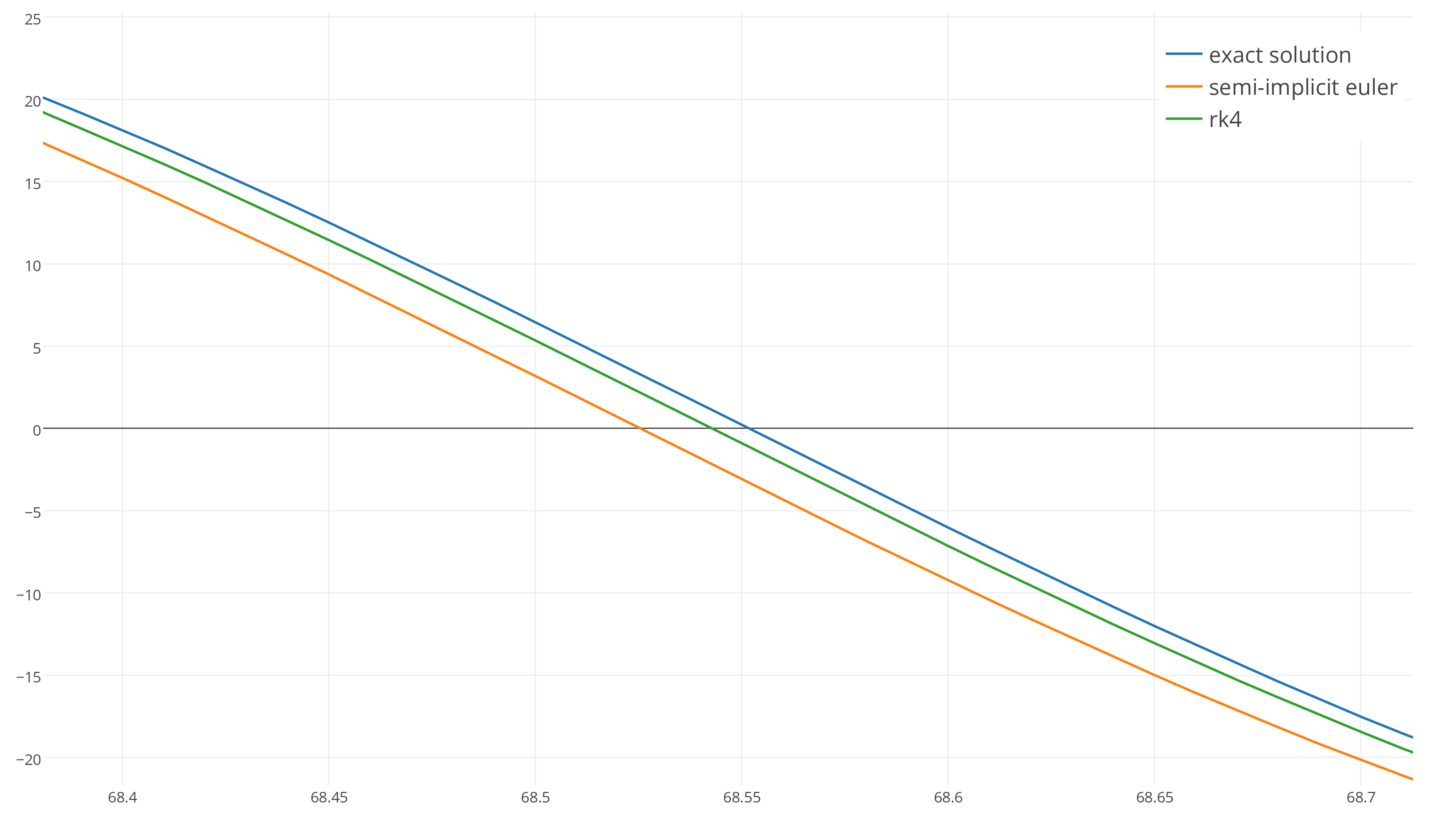
Now run the integrators for 90 seconds and zoom in:



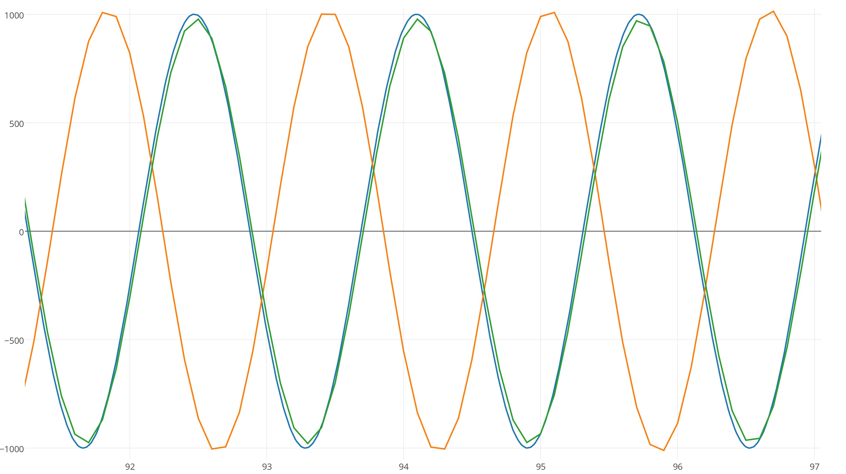
After 90 seconds, the Euler symplectic method (the orange curve) shifted in phase relative to the exact solution because its frequency was slightly different, while the green RK4 curve corresponds to the frequency, but loses energy!

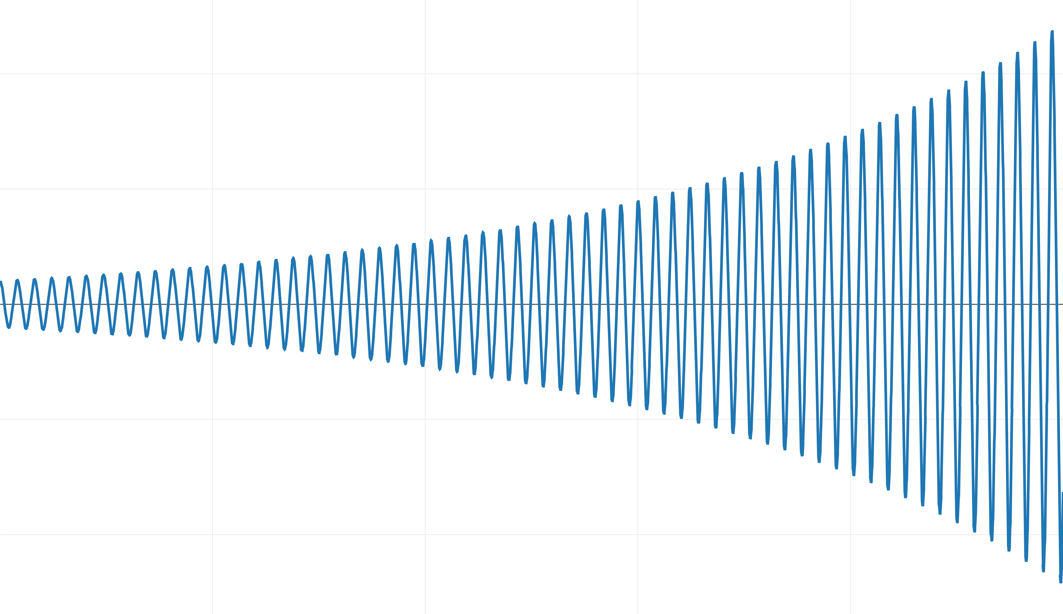
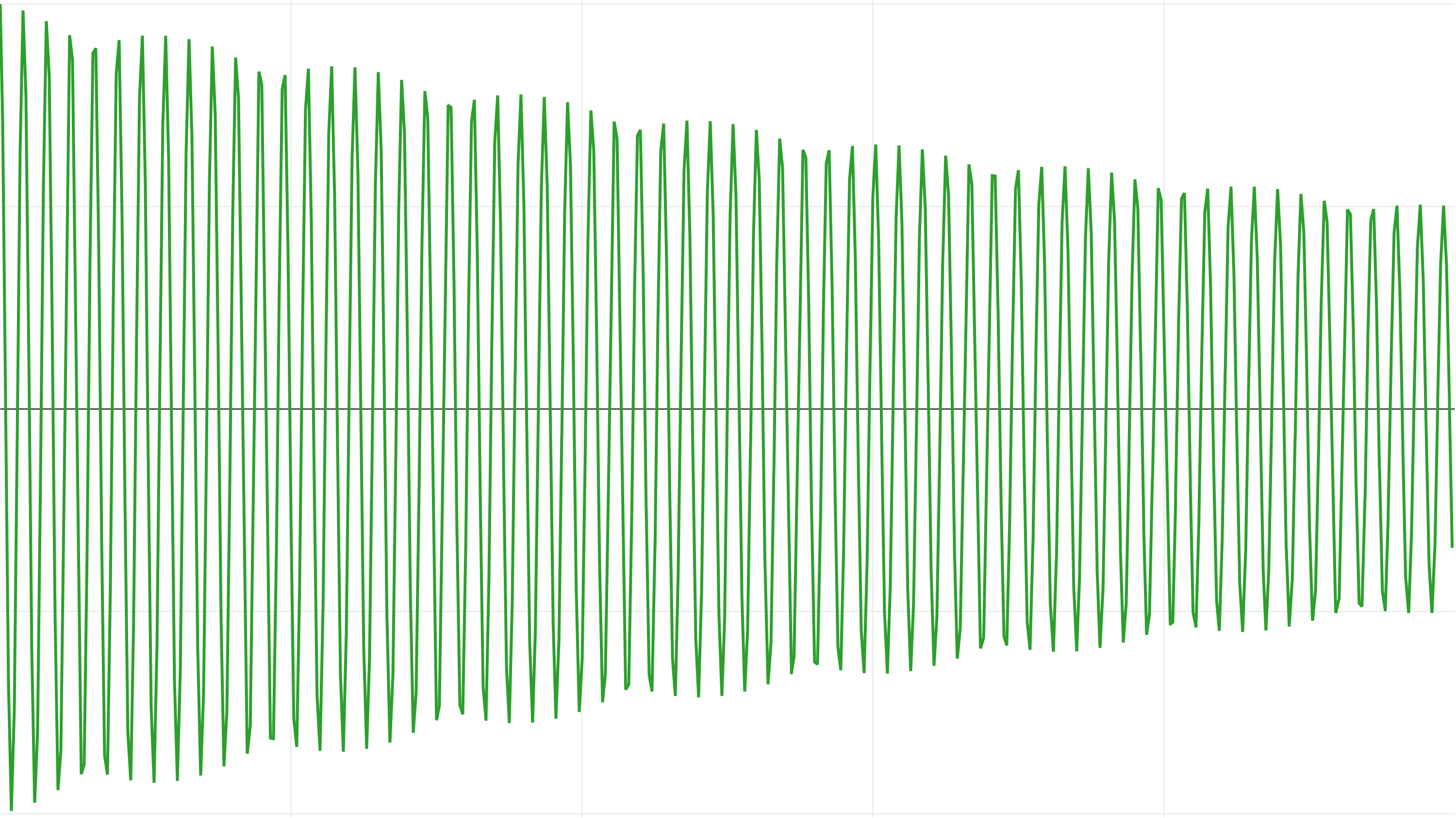
We can clearly notice this by increasing the time step to 0.25 seconds.

RK4 maintains the correct frequency, but loses energy:



And the Euler symplectic method on average saves energy much better:



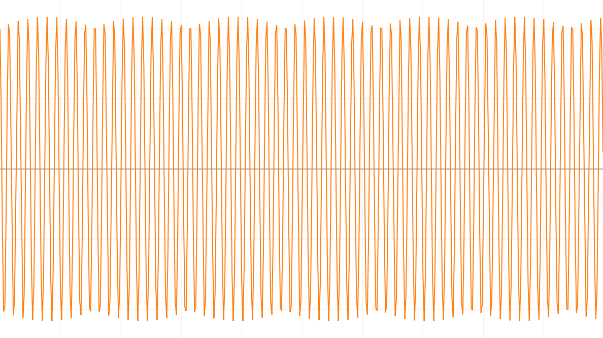
But from shifting from phase. What an interesting result! As you can see, if the RK4 has a higher order of accuracy, then it is not necessarily "better." There are many nuances in this matter.

Conclusion

We implemented three different integrators and compared the results.

1. Explicit Euler Method
2. The symplectic Euler method
3. Runge-Kutta Method of Order 4 (RK4)

So which integrator should be used in the game?

I recommend the sympathetic Euler method . It is “cheap” and simple to implement, much more stable than the explicit Euler method and, on average, tends to conserve energy even under close to extreme conditions.

If you really need more accuracy than the symplectic Euler method, I recommend looking at higher-order symplectic integrators designed for Hamiltonian systems . This way you will learn more advanced high-order integration techniques that are better suited for simulations than RK4.

And finally, if you are still writing in a game like this:

    position + = velocity * dt;
    velocity + = acceleration * dt;

Then spend a second and replace these lines with:

    velocity + = acceleration * dt;
    position + = velocity * dt;

Believe me, you will be happy about this.