Theoretical foundations of spline interpolation or why IQ tests have no solution

Good time, Habr!

A lot of time has passed since I wrote my first article , and almost a year from the moment I came up with the idea for the second. Due to many circumstances (primarily laziness and forgetfulness), this idea was never realized before, but now I got together, wrote all this material and am ready to present it to your attention.

I'll start with a small introduction. As a student of the 4th, at that time, undergraduate course, I studied the course “Computer Graphics”. There were a lot of different interesting (and not so) tasks, but one thing directly hit my soul: interpolation with cubic splines with the given first derivatives at the ends of the interval. The user had to set the values ​​of the first derivatives, and the program had to read and display the interpolation curve. The peculiarity and the main complexity of the task is that it is the first derivatives that are specified, and not the second ones, as in the classical formulation of spline interpolation.
How I solved it, and what it ultimately came to, I will just set out in this article. And yes, if according to the description of the task you didn’t understand its meaning, complexity, don’t worry, I’ll try to reveal all this as well. So let's go.

Oh no, wait a moment. Here are two numbers:
a) 2, 4, 6, 8 ,?
b) 1, 3 ,? , 7, 9

What numbers should stand in the place of questions and why? Are you really sure of your answer?

Interpolation

Interpolation, interpolation (from Latin inter-polis - “smoothed, updated, updated, transformed”) - in computational mathematics, a way of finding intermediate values ​​of a quantity from an available discrete set of known values. (c) Wikipedia

I will explain with examples. There are problems when we need to know, conditionally, the “distribution law" (I put it in quotation marks, since this, generally speaking, is a term from another area of ​​mathematics) of a certain parameter by several of its known values. Most often we are talking about a change in a parameter over time: the coordinates of a moving body, the temperature of an object, currency fluctuations, etc. Moreover, due to some circumstances, we did not have the opportunity to monitor this parameter continuously, we could recognize its values ​​only at some particular points in time. In this case, the source data is a set of points of the form value (time) , and the goal of the task is to restore the curve passing through these points and continuously describing the change in this parameter.

It should be understood that the impossibility of constant monitoring of the relevant parameter is usually some kind of technological limitation. With the development of technology, such situations are becoming less and less. Of the modern tasks of such a plan is the trajectory of movement, for example, of a rover. It is still not possible to maintain a continuous communication session (for now), but I want to control its movement and draw beautiful trajectories. It turns out that specific coordinates can be found only at those moments when the connection is still established, and the entire trajectory must be restored from the points thus obtained from time to time.
Another application of interpolation. Some modern TVs display images with a refresh rate of the picture to> = 1000Hz (although these are still outrageous values). Most TVs do not know how, but even so many display a picture at a frequency of 100 Hz - such a value is already quite a classic. And if you believe Wikipedia, then in the cinema "the frequency of 24 frames per second is the global standard." In order to turn 24 frames per second of the original video stream into 100 frames per second of the result, the TV uses interpolation. Namely, some algorithms in the style of “take two adjacent frames 1 and 2, calculate the difference between them and form 3 additional frames from it that need to be shoved between those two initial ones” -> frames 1, 1_1 , 1_2 are obtained, 1_3 , 2

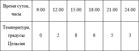
For further discussion, we take a simpler example. Imagine, for example, laboratory work on geography in some 6th grade (by the way, I once really had one). It is necessary to measure the air temperature every 3 hours and record data, and then pass the teacher a schedule of temperature changes versus time of day. Suppose, according to the results of measurements, we got such a plate (the data was invented randomly and does not pretend to any credibility):



Display the data on the chart:



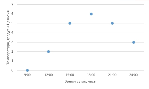
Actually, the data is recorded and reflected on the graph. We have come close to the problem of interpolation - how to restore a smooth curve from the available points?

Number of conditions and degree of interpolating polynomial

Can we generally guarantee that such a function that connects all given points exists at all?

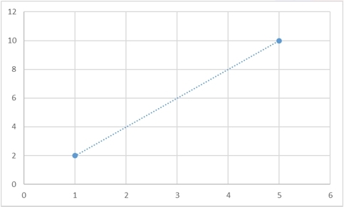
Yes, such a function is guaranteed to exist, and moreover, there will be infinitely many such functions. For any set of points, it will be possible to come up with as many as needed functions that will pass through them. And here are a few examples of how two points can be connected in different ways:





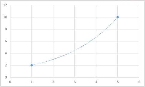
However, there is a way to set the interpolation curve uniquely. In the most classical case, the polynomial is taken as the interpolation curve:

$$

In order to draw such a polynomial through the available points in a unique way, it is necessary and sufficient that the degree of the polynomial is 1 less than the number of conditions (I specially highlighted this word, because at the end of this section I will return to this formulation). For now, for the sake of simplicity, the condition will be the coordinates of the point. In human language, through 2 points you can clearly draw a straight line (polynomial of the 1st degree), through 3 points - a parabola (polynomial of the 2nd degree), etc.

Returning to our problem with temperature - we identified 6 points in it, which means that in order to conduct a polynomial in a unique way, it must be of the 5th degree



The interpolating polynomial will then look like this:

$\$\; inline\; \$\; -\; \backslash \; frac\; \{x\; ^\; 5\}\; \{14580\}\; +\; \backslash \; frac\; \{13x\; ^\; 4\}\; \{1944\}\; -\; \backslash \; frac\; \{41x\; ^\; 3\}\; \{162\}\; +\; \backslash \; frac\; \{983x\; ^\; 2\}\; \{216\}\; -\; \backslash \; frac\; \{2273x\}\; \{60\}\; +\; 117\; \$\; inline\; \$$

And now, an important remark should be made and clarified what I meant by “condition” . A polynomial can be set not only by the coordinates of the points through which it passes, conditions can be any parameters of this polynomial. In the simplest case, these are really the coordinates of the points. But, as a condition, we can take, for example, the first derivative of this polynomial at some point. The second derivative. The third derivative. In general, any possible derivative at any of the points at which this polynomial exists. Let me explain with an example: A
straight line can be defined uniquely, as I said, by two points:



The same straight line, on the other hand, can be determined by the coordinate of one point and the angle of inclination of the alpha to the horizontal:



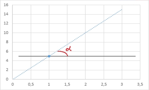
Polynomials of higher degrees can also use more complex conditions (second derivative, third derivative, etc.), and each such parameter will go into the general account of the number of conditions that uniquely determine this polynomial. In order not to be unfounded, here is another example:

Let us be given three conditions:

$$

Three conditions, then we want to get a polynomial of the second degree:

$$

Substitute $$

We consider the first derivative and consider $$

We count the second derivative and count $$

From here we get that our polynomial looks like this:

$$

Cubic Spline Interpolation

Here, quietly, we are getting to my task. Polynomial interpolation is not the only possible way of interpolation. Among all other methods, there is a method of interpolation with cubic splines.

The fundamental difference between the idea of ​​spline interpolation and interpolation by a polynomial is that there is only one polynomial, and the spline consists of several polynomials, namely, their number is equal to the number of intervals within which we interpolate. In the example with our air temperature, in which we have 6 points, we will have 5 intervals - accordingly, we will have 5 polynomials, each in its own interval.

Each of these polynomials is a polynomial of the third degree (strictly speaking, the degree is not higher than the third, since at some interval the interpolating curve can become a quadratic parabola or even a linear function, but in the general case it is still a polynomial of the third degree) . Writing the above formula, we get that all our points will be connected by a certain curve$$where everyone $$ Is a polynomial of the third degree, namely:

$$

Returning to what was said in the previous paragraph, in order to uniquely specify one polynomial of degree 3, 4 conditions are necessary. In this problem, we have 5 polynomials, that is, to set them all, we need a total of 5 ∙ 4 = 20 conditions. And here is how they are obtained:

1) The first polynomial is defined at the first and second points - these are two conditions. The second polynomial is defined at the second and third points - two more conditions. The third polynomial, fourth, fifth - each of them is defined on 2 points - in total this gives 10 conditions.

2) For each intermediate point from the set (and these are 4 points with times 12:00, 15:00, 18:00, 21:00), the condition must be satisfied that the first and second derivatives for the left and right polynomials must coincide. Formally:

$$

$$

$$

Two such conditions for each of the intermediate points give 8 more conditions. It should be added that we ask only the fact of equality itself, and what specific significance they take in doing so is a completely different task and it is considered quite difficult.

3) Two conditions remain that are not yet defined. These are the so-called “boundary conditions”, from the determination of which exactly which spline will turn out. Usually, the second derivatives at the ends of the interval are set to 0:

$$

$$

If we do this, then we will get the so-called “natural spline”. To calculate such splines, a huge number of libraries have already been written, take and use any.

The difference between my task and the classical statement of the problem, my thoughts on the task and the solution itself

And so we came to the condition of my task. The teacher came up with such a task that the first derivatives should be asked$$ and 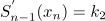$$at the left and right ends of the interval, and the program should read the interpolating curve. And for such a requirement, I did not find any ready-made algorithms ...
Of course, I will not describe your entire “creative” path from the moment I heard the task to before I passed it. I will only tell the idea itself and show its implementation.

The complexity of the task is that, setting the first derivatives at the ends of the interval, yes, we define this spline. In theory. But to calculate it in practice is a rather complicated and completely non-obvious task (anyone can see the code for finding a natural spline on Wiki - en.wikipedia.org/wiki/Cubic_spline- and try to understand him at least). Of course, I absolutely did not want to spend a lot of time digging into matan and trying to deduce the formulas I needed. I wanted a simpler and more elegant solution. And I found him.
Consider our spline and take the first of its intervals. On this interval, 3 conditions have already been set:

$$

$$

$$- set by the user.

In order to uniquely define a cubic polynomial on this interval, we need one more condition. But we can just come up with it! Take the second derivative and set it equal, for example, 0:

$$- an unfounded assumption.

Thus, knowing these 4 conditions, we completely determine this polynomial. Knowing all the parameters of this polynomial, we can calculate the values ​​of the first and second derivatives at the second point, and since they coincide with the values ​​of the first and second derivatives for the polynomial in the second interval, this leads to the fact that we also determine the second polynomial:

$$

$$

$$ - calculated from $$

$$ - calculated from $$

Similarly, we consider the third polynomial, the fourth, fifth, and so on, no matter how many there are. That is, in fact, we recreate the entire spline. But since we took$$ completely randomly, this will lead to the derivative $$set by the user on the right end of the spline will not coincide with the derivative $$, which we obtained during such calculations. But it turns out that the meaning of the derivative$$ at the right end of the spline is a function that depends on the value of the second derivative $$ on the left end:

$$

And since such a spline, which would satisfy the given conditions, is guaranteed to exist, and exists in a single copy, this means that we can consider the difference:

$$

and try to find that value $$at which $$would go to 0 - and that would be the right value$$that builds the spline the user is looking for: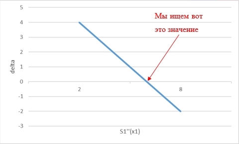



The most remarkable thing in my idea is that this dependence turned out to be linear (regardless of the number of points through which we draw the spline. This fact is proved by theoretical calculations), which means that you can randomly take any two initial values $$ and $$count $$ and $$, and immediately calculate the very correct value that the desired spline will build for us:

$$

Total, we are guaranteed to find the desired spline for 3 runs of such calculations.

Some code and screenshots of the program

class CPoint
{
    public int X { get; }
    public int Y { get; }
    public double Df { get; set; }
    public double Ddf { get; set; }
    public CPoint(int x, int y)
    {
        X = x;
        Y = y;
    }
}

class CSplineSubinterval
{
    public double A { get; }
    public double B { get; }
    public double C { get; }
    public double D { get; }
    private readonly CPoint _p1;
    private readonly CPoint _p2;
    public CSplineSubinterval(CPoint p1, CPoint p2, double df, double ddf)
    {
        _p1 = p1;
        _p2 = p2;
        B = ddf;
        C = df;
        D = p1.Y;
        A = (_p2.Y - B * Math.Pow(_p2.X - _p1.X, 2) - C * (_p2.X - _p1.X) - D) / Math.Pow(_p2.X - _p1.X, 3);
    }
    public double F(int x)
    {
        return A * Math.Pow(x - _p1.X, 3) + B * Math.Pow(x - _p1.X, 2) + C * (x - _p1.X) + D;
    }
    public double Df(int x)
    {
        return 3 * A * Math.Pow(x - _p1.X, 2) + 2 * B * (x - _p1.X) + C;
    }
    public double Ddf(int x)
    {
        return 6 * A * (x - _p1.X) + 2 * B;
    }
}

class CSpline
{
    private readonly CPoint[] _points;
    private readonly CSplineSubinterval[] _splines;
    public double Df1
    {
        get { return _points[0].Df; }
        set { _points[0].Df = value; }
    }
    public double Ddf1
    {
        get { return _points[0].Ddf; }
        set { _points[0].Ddf = value; }
    }
    public double Dfn
    {
        get { return _points[_points.Length - 1].Df; }
        set { _points[_points.Length - 1].Df = value; }
    }
    public double Ddfn
    {
        get { return _points[_points.Length - 1].Ddf; }
        set { _points[_points.Length - 1].Ddf = value; }
    }
    public CSpline(CPoint[] points)
    {
        _points = points;
        _splines = new CSplineSubinterval[points.Length - 1];
    }
    public void GenerateSplines()
    {
        const double x1 = 0;
        var y1 = BuildSplines(x1);
        const double x2 = 10;
        var y2 = BuildSplines(x2);
        _points[0].Ddf = -y1 * (x2 - x1) / (y2 - y1);
        BuildSplines(_points[0].Ddf);
        _points[_points.Length - 1].Ddf = _splines[_splines.Length - 1].Ddf(_points[_points.Length - 1].X);
    }
    private double BuildSplines(double ddf1)
    {
        double df = _points[0].Df, ddf = ddf1;
        for (var i = 0; i < _splines.Length; i++)
        {
            _splines[i] = new CSplineSubinterval(_points[i], _points[i + 1], df, ddf);
            df = _splines[i].Df(_points[i + 1].X);
            ddf = _splines[i].Ddf(_points[i + 1].X);
            if (i < _splines.Length - 1)
            {
                _points[i + 1].Df = df;
                _points[i + 1].Ddf = ddf;
            }
        }
        return df - Dfn;
    }
}

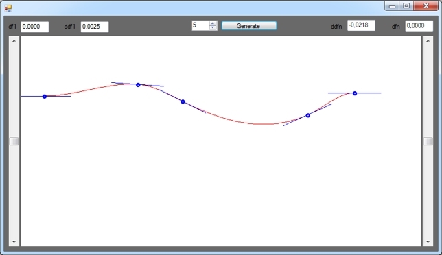
Blue segments are the first derivatives of a spline at its corresponding points. Added such a graphic element for greater clarity.

Advantages and disadvantages of the algorithm

Frankly, I did not conduct any serious analysis. It would be nice to write tests, check how it works under different conditions (few / many interpolation points, equal / arbitrary between points, linear / square / cubic / trigonometric / etc. Functions, etc.), but I didn’t do this excuse me :)

Offhand you can say that the complexity of the algorithm is O (N), since, as I said, regardless of the number of points, two runs of calculations are enough to get the correct value of the second derivative at the left end of the interval, and one more to build a spline.

However, if someone wants to delve into the code and conduct some more detailed analysis of this algorithm, I will only be glad. Write to me except about the results, I would be interested.

So what are the IQ tests to blame for?

At the very beginning of the article, I wrote two number series and asked them to continue. This is a fairly common question in all kinds of IQ tests. In principle, the question is like a question, but if you dig a little deeper, it turns out that it is rather delusional, because with some desire you can prove that there is no “right” answer to it.

Let's start with a series of “2, 4, 6, 8,?”
Imagine this number series as a set of pairs of values$$:



where as $$ we take the number itself, and as $$- serial number of this number. What value should be in place$$?

The thought that I am trying to smoothly bring to is that we can substitute absolutely any value. After all, what actually check such tasks? The ability of a person to find a certain rule that connects all available numbers, and according to this rule to deduce the next number in a sequence. In scientific terms, the problem here is extrapolation (the task of interpolation is to find a curve passing through all points within a certain interval, and the task of extrapolation is to continue this curve beyond the limits of the interval, thus “predicting” the behavior of the curve in the future). So, extrapolation does not have a definite solution. At all. Never. If it were otherwise, people would have predicted the weather forecast for the whole history of mankind ahead of time, and ruble exchange rates would never be a surprise.

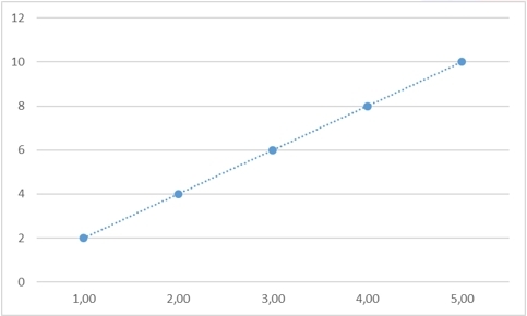
Of course, it is assumed that the correct answer in this problem is still there and it is 10, and then the “law" connecting all these numbers is $$



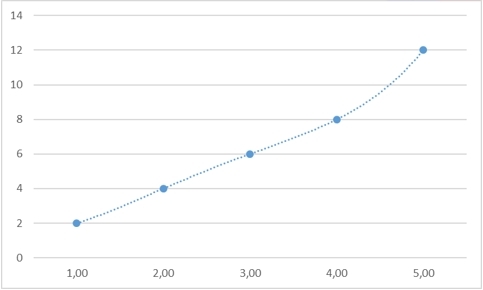
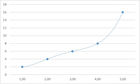
However, we take any other meaning - and we can also find a law that justifies it:

$$


$$


$$


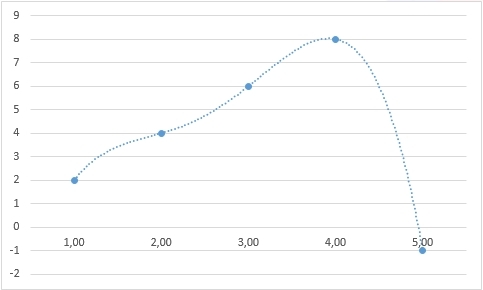
Well, with the extrapolation sorted out, it does not have a definite solution, even theoretically. But maybe we can find the missing number in the second row?



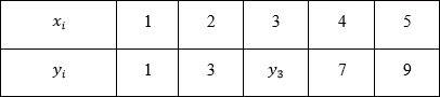
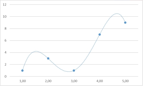
I believe the right answer $$. Who can challenge? :)

$$

Git repository

Last time, I was scolded for posting the project as an archive in the cloud, and not as codes in the repository, so this time I correct this error: github.com/WieRuindl/Splines