February 6, 2017 at 08:38
Interesting clustering algorithms, part one: Affinity propagation
Part One - Affinity Propagation
Part Two - DBSCAN
Part Three - Time Series Clustering
Part Four - Self-Organizing Maps (SOM)
Part Five - Growing Neural Gas (GNG)
If you ask a novice data analyst what classification methods he knows, you will probably be listed a pretty decent list: statistics, trees, SVMs, neural networks ... But if you ask about clustering methods, in return you will most likely get a confident “k-means!” It is this golden hammer that is considered in all machine learning courses. Often, it does not even come to its modifications (k-medians) or connected graph methods.
Not that k-means is so bad, but its result is almost always cheap and angry. There are more perfectclustering methods, but not everyone knows what to use when, and very few understand how they work. I would like to open the veil of secrecy over some algorithms. Let's start with Affinity propagation.
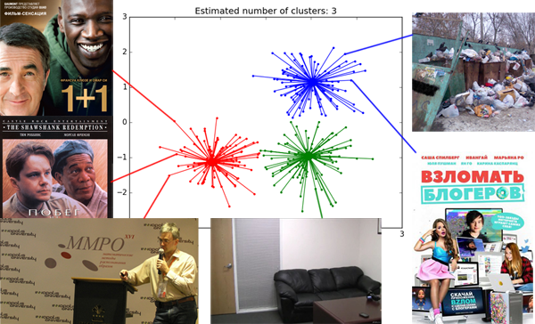
It is assumed that you are familiar with the classification of clustering methods , and also have already used k-means and know its pros and cons. I will try not to go very deep into the theory, but try to convey the idea of the algorithm in simple language.
Affinity propagation (AP, aka proximity distribution method) receives an input matrix of similarity between the elements of the dataset and returns the set of labels assigned to these elements. Without further ado, I'll immediately lay out the algorithm on the table:
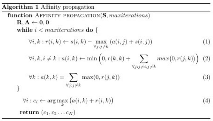
Ha, it would be something to spread. Only three lines, if we consider the main cycle; (4) - explicit labeling rule. But not so simple. Most programmers are not at all clear what these three lines do with matrices ,
,  and
and  . A near-official article explains that and - matrices of “responsibility” and “availability”, respectively, and that in the cycle there is a “messaging” between potential cluster leaders and other points. Honestly, this is a very superficial explanation, and it is not clear whether the purpose of these matrices is how or why their values change. Trying to figure it out will most likely lead you somewhere here . It’s a good article, but it’s hard for an unprepared person to withstand a whole monitor screen clogged with formulas.
So I will start from the other end.
In some space, in some state, dots live. The dots have a rich inner world, but there is some rule by which they can tell how similar their neighbor is. Moreover, they already have a tablewhere everything is written and she almost never changes.
It’s boring to be alone in the world, so the points want to get together in hobby groups. Circles are formed around the leader (exemplar), who represents the interests of all members of the partnership. Each point would like to see the leader of someone who is as similar to her as possible, but is ready to put up with other candidates if many others like them. It should be added that the points are rather modest: everyone thinks that someone else should be the leader. You can reformulate their low self-esteem as follows: each point believes that when it comes to grouping, it does not look like itself ( ) Convincing a point to become a leader can be either collective encouragement from comrades similar to it, or, conversely, if there is absolutely no one like it in society.
The points do not know in advance what kind of teams they will be, nor their total number. The union goes from top to bottom: at first the points cling to the presidents of the groups, then they only reflect on who else supports the same candidate. Three parameters influence the choice of a point as a leader: similarity (it has already been said about it), responsibility and accessibility. Responsibility (responsibility, table with elements  ) is responsible for how
  wants to see
  his leader. Responsibility is assigned by each point to the candidate for group leaders. Availability (availability, table, with elements
  ) - there is a response from a potential leader , how good ready to represent interests . Responsibility and accessibility points are calculated, including for themselves. Only when there is great self-responsibility (yes, I want to represent my interests) and self-availability (yes, I can represent my interests), i.e.
 , a point can overcome innate self-doubt. Ordinary points eventually join the leader for which they have the highest amount
 . Usually at the very beginning,
 and
and  .
.
Let's take a simple example: points X, Y, Z, U, V, W, whose whole inner world is love for cats, . X is allergic to cats, for him we will take
 , Y treats them cool,
  , and Z is simply not up to them,
  . U has four cats at home (
 ), V has five (
 ), and W has as many as forty (
 ) Define dissimilarity as the absolute value of the difference. X is unlike Y by one conditional point, and by U - by as much as six. Then the similarities,- it's just a minus of dissimilarity. It turns out that the points with zero similarity are exactly the same; the more negative, the stronger the points differ . A bit counterintuitive, but oh well. The size of "self-dissimilarity" in the example is estimated at 2 points (
 )
)
So, in the first step, every point blames everyone (including oneself) in proportion to the similarity between and and inversely proportional to the similarity betweenand the most similar vector except ((1) c  ) Thus:
If then would like was her representative.
  means that she wants to be the founder of a team
  - what wants to belong to another team.
Returning to an example: X holds Y liable in the amount of point, on Z -
  point, on U -
  but on yourself . X, in general, does not mind that the leader of the hate group was Z if Y does not want to be him, but is unlikely to communicate with U and V, even if they assemble a large team. W is so unlike all other points that there is nothing left for it but to assign responsibility in the amount of
 point only on yourself.
Then the points begin to think how ready they are to be a leader (available, available, for leadership). Accessibility for oneself (3) consists of all positive responsibility, “votes” given to the point. Forit doesn’t matter how many points they think that it will be bad to represent them. For her, the main thing is that at least someone thinks that she will represent them well. Availability for depends on how much I’m ready to represent myself and the number of positive reviews about him (2) (someone else also believes that he will be an excellent representative of the team). This value is limited from above to zero to reduce the influence of points about which too many think well, so that they do not combine even more points into one group and the cycle does not get out of control. Less the more votes you need to collect to was equal to 0 (i.e., this point was not against taking under its wing also )
A new round of elections begins, but now . Recall that
 , a
, a  . This has a different effect on
Accessibility leaves points in the competition that are either ready to stand up for themselves (W, , but this does not affect (1), since even taking into account the correction, W is located very far from other points) or those that others are ready to stand for (Y, in (3) she has in terms of the summand of X and Z). X and Z, who are not strictly the best resemble someone, but still look like someone, are eliminated from the competition. This affects the distribution of liability, which affects the distribution of availability and so on. In the end, the algorithm stops -stop changing. X, Y and Z team up around Y; friends of U and V with U as a leader; W well and with 40 cats.
We rewrite the decision rule to get another look at the decision rule of the algorithm. We use (1) and (3). We denote - similarity adjusted for the fact that talks about his commanding abilities ;
  - dissimilarity - as amended.
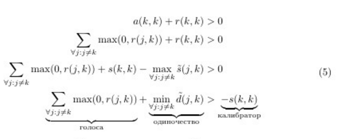
Approximately what I formulated at the beginning. It can be seen from this that the less confident the points are, the more “votes” must be gathered, or the more unlike the others you need to be in order to become a leader. Those. less , the larger the groups are.
Well, I hope you have acquired some intuitive insight into how the method works. Now a little more serious. Let's talk about the nuances of applying the algorithm.
Clustering can be represented as a discrete maximization problem with constraints. Let the similarity function be given on the set of elements . Our task is to find such a vector of labels
 which maximizes the function
Where - term limiter equal
  if there is a point that chose the point their leader (
 ), but herself does not consider himself a leader (
 ) Bad news: finding the perfect
 - This is an NP-complex problem, known as the object placement problem. Nevertheless, for its solution there are several approximate algorithms. In the methods of interest to us
 ,
,  and
and  They are represented by the vertices of a bipartite graph, after which information is exchanged between them, allowing, from a probabilistic point of view, to assess which label is best suited for each element. See the conclusion here . About distribution of messages in bipartite graphs see here . In general, the distribution of proximity is a special case (rather, narrowing) of the cyclic distribution of beliefs (loopy belief propagation, LBP, see here ), but instead of the sum of the probabilities (Sum-Product subtype) in some places we take only the maximum (Max-Product subtype) of them. Firstly, LBP-Sum-Product is an order of magnitude more complicated, secondly, it is easier to run into computational problems there, and thirdly, theorists say that this makes more sense for the clustering problem.
The authors of AP talk a lot about "messages" from one element of the graph to another. This analogy comes from the derivation of formulas through the dissemination of information in a graph. In my opinion, it is a little confusing, because in the implementations of the algorithm there are no point-to-point messages, but there are three matrices, and . I would suggest the following interpretation:
Affinity propagation is deterministic. He has difficulty where
where  - the size of the data set, and
  - the number of iterations, and takes
  memory. There are modifications of the algorithm for sparse data, but still, the AP becomes very sad with the increase in the size of the dataset. This is a pretty serious flaw. But the spread of proximity does not depend on the dimension of data elements. There is no parallelized version of AP yet. The trivial parallelization in the form of a set of algorithm starts is not suitable due to its determinism. In the official FAQ , it is written that there are no options with the addition of real-time data, but I found this article.
There is an accelerated version of AP. The method proposed in the article is based on the idea that it is not necessary to calculate all updates to the matrices of accessibility and responsibility in general, because all points in the thick of other points relate to distant copies from them approximately the same.
If you want to experiment (keep it up!), I would suggest conjuring over formulas (1-5). Parts they look suspiciously like neural-grid ReLu. I wonder what happens if you use ELu. In addition, since you now understand the essence of what is happening in the cycle, you can add additional members to the formulas that are responsible for the behavior you need. Thus, you can “push” the algorithm towards clusters of a certain size or shape. It is also possible to impose additional restrictions if it is known that some elements are more likely to belong to one set. However, this is speculation.
Affinity propagation, like many other algorithms, can be interrupted early if and stop updating. For this, almost all implementations use two values: the maximum number of iterations and the period with which the value of updates is checked.
Affinity propagation is prone to computational oscillations in cases where there are some good clustering. To avoid problems, firstly, at the very beginning a little noise is added to the similarity matrix (very, very little, so as not to affect determinism, in sklearn implementation of the order ), and secondly, when updating and used is not a simple assignment, and the assignment to the exponentially smoothing . The second optimization, in general, has a good effect on the quality of the result, but because of it, the number of necessary iterations increases. Authors suggest using a smoothing option.
 with default value in
  . If the algorithm does not converge or partially converges , increase
 before
  or before
  with a corresponding increase in the number of iterations.
This is what a failure looks like - a bunch of small clusters surrounded by a ring of medium-sized clusters:
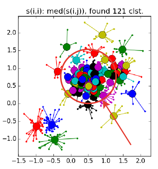
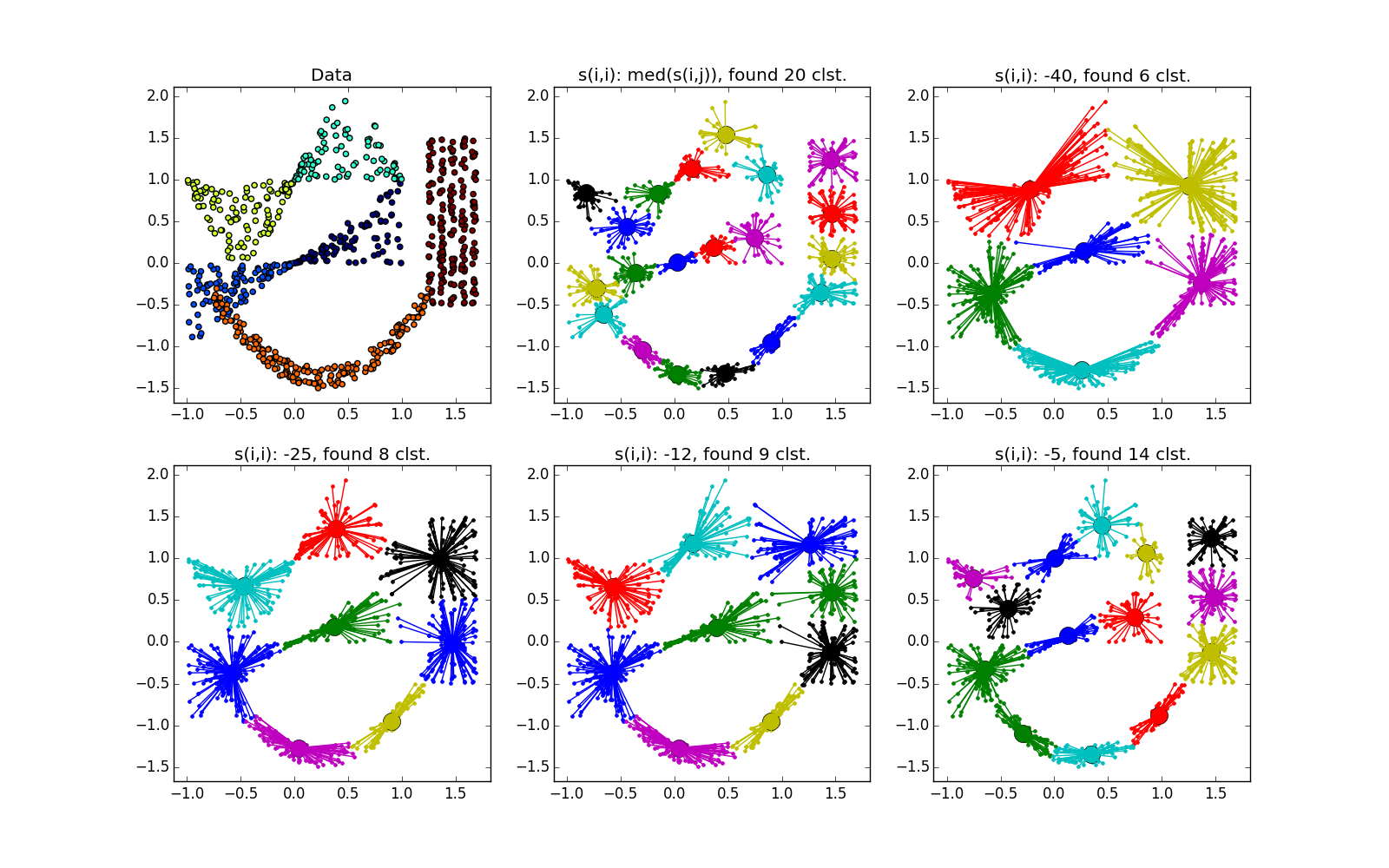
As already mentioned, instead of a predetermined number of clusters, the parameter “self-similarity” is used; less, the larger the clusters. There are heuristics for automatically adjusting the value of this parameter: use the median for allUsed for about ng bigger number of clusters; 25th percentile , or even a minimum of- for less (you still have to customize, ha ha). If the “self-similarity” value is too small or too large, the algorithm will not produce any useful results at all.
As it goes without saying to use the negative Euclidean distance between and  but no one restricts you in the choice. Even in the case of a dataset from vectors of real numbers, you can try a lot of interesting things. In general, the authors argue that the function of similarity is not imposed any special restrictions ; it’s not even necessary that the symmetry rule or the triangle rule is fulfilled. But it’s worth noting that the more ingenious you have, the less likely the algorithm will converge to something interesting.
The sizes of clusters obtained during the propagation of proximity vary within rather small limits, and if the dataset contains clusters of very different sizes, AP can either skip small ones or count large ones for several. Usually the second situation is less unpleasant - it is fixable. Therefore, often AP needs post-processing - additional clustering of group leaders . Any other method is suitable; additional information about the task can help here. It should be remembered that honest, lonely-standing points stand out for their clusters; such emissions should be filtered out before post-processing.
Fuh, the wall of text has ended, the wall of pictures has begun. Let's test Affinity propagation on different types of clusters.
Use affinity propagation when
Allegedly , various scientists have successfully used affinity propagation to
In all these cases, the result was better than with k-means. Not that it’s some kind of super result in itself. I do not know whether in all these cases a comparison was made with other algorithms. I plan to do this in future articles. Apparently, on datasets from real life, the ability to spread proximity to deal with clusters of different geometric shapes helps the most.
Well, that’s all. Next time, consider another algorithm and compare it with the proximity propagation method. Good luck, Habr!
Part Two - DBSCAN
Part Three - Time Series Clustering
Part Four - Self-Organizing Maps (SOM)
Part Five - Growing Neural Gas (GNG)
If you ask a novice data analyst what classification methods he knows, you will probably be listed a pretty decent list: statistics, trees, SVMs, neural networks ... But if you ask about clustering methods, in return you will most likely get a confident “k-means!” It is this golden hammer that is considered in all machine learning courses. Often, it does not even come to its modifications (k-medians) or connected graph methods.
Not that k-means is so bad, but its result is almost always cheap and angry. There are more perfectclustering methods, but not everyone knows what to use when, and very few understand how they work. I would like to open the veil of secrecy over some algorithms. Let's start with Affinity propagation.
It is assumed that you are familiar with the classification of clustering methods , and also have already used k-means and know its pros and cons. I will try not to go very deep into the theory, but try to convey the idea of the algorithm in simple language.
Affinity propagation
Affinity propagation (AP, aka proximity distribution method) receives an input matrix of similarity between the elements of the dataset
and returns the set of labels assigned to these elements. Without further ado, I'll immediately lay out the algorithm on the table:Ha, it would be something to spread. Only three lines, if we consider the main cycle; (4) - explicit labeling rule. But not so simple. Most programmers are not at all clear what these three lines do with matrices
, and . A near-official article explains that and - matrices of “responsibility” and “availability”, respectively, and that in the cycle there is a “messaging” between potential cluster leaders and other points. Honestly, this is a very superficial explanation, and it is not clear whether the purpose of these matrices is how or why their values change. Trying to figure it out will most likely lead you somewhere here . It’s a good article, but it’s hard for an unprepared person to withstand a whole monitor screen clogged with formulas. So I will start from the other end.
Intuitive explanation
In some space, in some state, dots live. The dots have a rich inner world, but there is some rule
by which they can tell how similar their neighbor is. Moreover, they already have a tablewhere everything is written and she almost never changes. It’s boring to be alone in the world, so the points want to get together in hobby groups. Circles are formed around the leader (exemplar), who represents the interests of all members of the partnership. Each point would like to see the leader of someone who is as similar to her as possible, but is ready to put up with other candidates if many others like them. It should be added that the points are rather modest: everyone thinks that someone else should be the leader. You can reformulate their low self-esteem as follows: each point believes that when it comes to grouping, it does not look like itself (
) Convincing a point to become a leader can be either collective encouragement from comrades similar to it, or, conversely, if there is absolutely no one like it in society. The points do not know in advance what kind of teams they will be, nor their total number. The union goes from top to bottom: at first the points cling to the presidents of the groups, then they only reflect on who else supports the same candidate. Three parameters influence the choice of a point as a leader: similarity (it has already been said about it), responsibility and accessibility. Responsibility (responsibility, table
with elements ) is responsible for how wants to see his leader. Responsibility is assigned by each point to the candidate for group leaders. Availability (availability, table, with elements ) - there is a response from a potential leader , how good ready to represent interests . Responsibility and accessibility points are calculated, including for themselves. Only when there is great self-responsibility (yes, I want to represent my interests) and self-availability (yes, I can represent my interests), i.e., a point can overcome innate self-doubt. Ordinary points eventually join the leader for which they have the highest amount. Usually at the very beginning, and . Let's take a simple example: points X, Y, Z, U, V, W, whose whole inner world is love for cats,
. X is allergic to cats, for him we will take, Y treats them cool, , and Z is simply not up to them, . U has four cats at home (), V has five (), and W has as many as forty () Define dissimilarity as the absolute value of the difference. X is unlike Y by one conditional point, and by U - by as much as six. Then the similarities,- it's just a minus of dissimilarity. It turns out that the points with zero similarity are exactly the same; the more negative, the stronger the points differ . A bit counterintuitive, but oh well. The size of "self-dissimilarity" in the example is estimated at 2 points () So, in the first step, every point
blames everyone (including oneself) in proportion to the similarity between and and inversely proportional to the similarity betweenand the most similar vector except ((1) c ) Thus:- The nearest (most similar) point defines the distribution of responsibility for all other points. The location of points farther than the first two so far only affects allotted to them and only to them.
- Responsibility assigned to the nearest point also depends on the location of the second nearest.
- If within reach there are several candidates who are more or less similar to him; those will be assigned approximately the same responsibility
- acts as a kind of limiter - if a point is too much unlike all the others, it has nothing left to do but to rely only on itself
If
then would like was her representative. means that she wants to be the founder of a team - what wants to belong to another team. Returning to an example: X holds Y liable in the amount of
point, on Z - point, on U - but on yourself . X, in general, does not mind that the leader of the hate group was Z if Y does not want to be him, but is unlikely to communicate with U and V, even if they assemble a large team. W is so unlike all other points that there is nothing left for it but to assign responsibility in the amount ofpoint only on yourself. Then the points begin to think how ready they are to be a leader (available, available, for leadership). Accessibility for oneself (3) consists of all positive responsibility, “votes” given to the point. For
it doesn’t matter how many points they think that it will be bad to represent them. For her, the main thing is that at least someone thinks that she will represent them well. Availability for depends on how much I’m ready to represent myself and the number of positive reviews about him (2) (someone else also believes that he will be an excellent representative of the team). This value is limited from above to zero to reduce the influence of points about which too many think well, so that they do not combine even more points into one group and the cycle does not get out of control. Lessthe more votes you need to collect to was equal to 0 (i.e., this point was not against taking under its wing also ) A new round of elections begins, but now
. Recall that, a . This has a different effect on . Then does not play a role, and in (1) everything
  on the right side will be no less than they were in the first step.
  essentially moves the point away from . The point’s self-responsibility rises from the fact that the best candidate, from her point of view, has bad reviews.
 . Both effects appear here. This case splits into two:
 - max. The same as in case 1, but the responsibility assigned to the point increases
 - max. Then will be no more than in the first step, decreases. If we continue the analogy, it is as if the point, which was already considering whether to become its leader, received additional approval.
Accessibility leaves points in the competition that are either ready to stand up for themselves (W,
, but this does not affect (1), since even taking into account the correction, W is located very far from other points) or those that others are ready to stand for (Y, in (3) she has in terms of the summand of X and Z). X and Z, who are not strictly the best resemble someone, but still look like someone, are eliminated from the competition. This affects the distribution of liability, which affects the distribution of availability and so on. In the end, the algorithm stops -stop changing. X, Y and Z team up around Y; friends of U and V with U as a leader; W well and with 40 cats. We rewrite the decision rule to get another look at the decision rule of the algorithm. We use (1) and (3). We denote
- similarity adjusted for the fact that talks about his commanding abilities ; - dissimilarity - as amended.Approximately what I formulated at the beginning. It can be seen from this that the less confident the points are, the more “votes” must be gathered, or the more unlike the others you need to be in order to become a leader. Those. less
, the larger the groups are. Well, I hope you have acquired some intuitive insight into how the method works. Now a little more serious. Let's talk about the nuances of applying the algorithm.
A very, very brief excursion into theory
Clustering can be represented as a discrete maximization problem with constraints. Let the similarity function be given on the set of elements
. Our task is to find such a vector of labelswhich maximizes the function
Where
- term limiter equal if there is a point that chose the point their leader (), but herself does not consider himself a leader () Bad news: finding the perfect- This is an NP-complex problem, known as the object placement problem. Nevertheless, for its solution there are several approximate algorithms. In the methods of interest to us, and They are represented by the vertices of a bipartite graph, after which information is exchanged between them, allowing, from a probabilistic point of view, to assess which label is best suited for each element. See the conclusion here . About distribution of messages in bipartite graphs see here . In general, the distribution of proximity is a special case (rather, narrowing) of the cyclic distribution of beliefs (loopy belief propagation, LBP, see here ), but instead of the sum of the probabilities (Sum-Product subtype) in some places we take only the maximum (Max-Product subtype) of them. Firstly, LBP-Sum-Product is an order of magnitude more complicated, secondly, it is easier to run into computational problems there, and thirdly, theorists say that this makes more sense for the clustering problem.The authors of AP talk a lot about "messages" from one element of the graph to another. This analogy comes from the derivation of formulas through the dissemination of information in a graph. In my opinion, it is a little confusing, because in the implementations of the algorithm there are no point-to-point messages, but there are three matrices
, and . I would suggest the following interpretation:- When calculating messages from data points are being sent to potential leaders - we look through matrices and along the lines
- When calculating messages are being sent from potential leaders to all other points - we look through matrices and along the columns
Affinity propagation is deterministic. He has difficulty
where - the size of the data set, and - the number of iterations, and takes memory. There are modifications of the algorithm for sparse data, but still, the AP becomes very sad with the increase in the size of the dataset. This is a pretty serious flaw. But the spread of proximity does not depend on the dimension of data elements. There is no parallelized version of AP yet. The trivial parallelization in the form of a set of algorithm starts is not suitable due to its determinism. In the official FAQ , it is written that there are no options with the addition of real-time data, but I found this article. There is an accelerated version of AP. The method proposed in the article is based on the idea that it is not necessary to calculate all updates to the matrices of accessibility and responsibility in general, because all points in the thick of other points relate to distant copies from them approximately the same.
If you want to experiment (keep it up!), I would suggest conjuring over formulas (1-5). Parts
they look suspiciously like neural-grid ReLu. I wonder what happens if you use ELu. In addition, since you now understand the essence of what is happening in the cycle, you can add additional members to the formulas that are responsible for the behavior you need. Thus, you can “push” the algorithm towards clusters of a certain size or shape. It is also possible to impose additional restrictions if it is known that some elements are more likely to belong to one set. However, this is speculation.Mandatory optimizations and parameters
Affinity propagation, like many other algorithms, can be interrupted early if
and stop updating. For this, almost all implementations use two values: the maximum number of iterations and the period with which the value of updates is checked. Affinity propagation is prone to computational oscillations in cases where there are some good clustering. To avoid problems, firstly, at the very beginning a little noise is added to the similarity matrix (very, very little, so as not to affect determinism, in sklearn implementation of the order
), and secondly, when updating and used is not a simple assignment, and the assignment to the exponentially smoothing . The second optimization, in general, has a good effect on the quality of the result, but because of it, the number of necessary iterations increases. Authors suggest using a smoothing option. with default value in . If the algorithm does not converge or partially converges , increase before or before with a corresponding increase in the number of iterations. This is what a failure looks like - a bunch of small clusters surrounded by a ring of medium-sized clusters:
As already mentioned, instead of a predetermined number of clusters, the parameter “self-similarity” is used
; less, the larger the clusters. There are heuristics for automatically adjusting the value of this parameter: use the median for allUsed for about ng bigger number of clusters; 25th percentile , or even a minimum of- for less (you still have to customize, ha ha). If the “self-similarity” value is too small or too large, the algorithm will not produce any useful results at all. As
it goes without saying to use the negative Euclidean distance between and but no one restricts you in the choice. Even in the case of a dataset from vectors of real numbers, you can try a lot of interesting things. In general, the authors argue that the function of similarity is not imposed any special restrictions ; it’s not even necessary that the symmetry rule or the triangle rule is fulfilled. But it’s worth noting that the more ingenious you have, the less likely the algorithm will converge to something interesting. The sizes of clusters obtained during the propagation of proximity vary within rather small limits, and if the dataset contains clusters of very different sizes, AP can either skip small ones or count large ones for several. Usually the second situation is less unpleasant - it is fixable. Therefore, often AP needs post-processing - additional clustering of group leaders . Any other method is suitable; additional information about the task can help here. It should be remembered that honest, lonely-standing points stand out for their clusters; such emissions should be filtered out before post-processing.
The experiments
Fuh, the wall of text has ended, the wall of pictures has begun. Let's test Affinity propagation on different types of clusters.
Wall of pictures
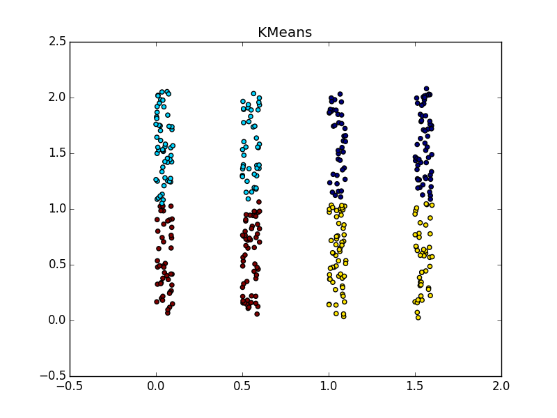
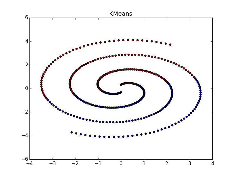
Распространение близости неплохо работает на кластерах в виде складок размерности меньше размерности данных. AP обычно не выделяет всю складку, а разбивает её на мелкие куски-субкластеры, которые потом придётся склеивать воедино. Впрочем, это не так уже и сложно: с двадцатью точками это проще, чем с двадцатью тысячами, плюс у нас есть дополнительная информация о вытянутости кластеров. Это намного лучше, чем k-means и многие другие неспециализированные алгоритмы.
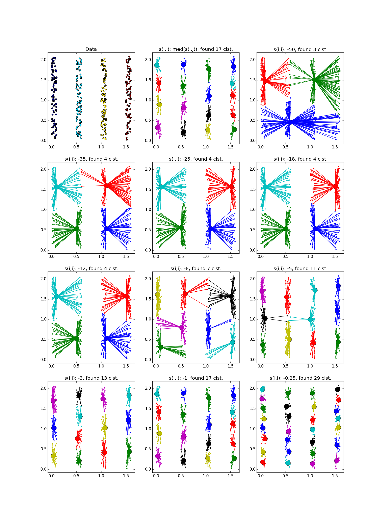
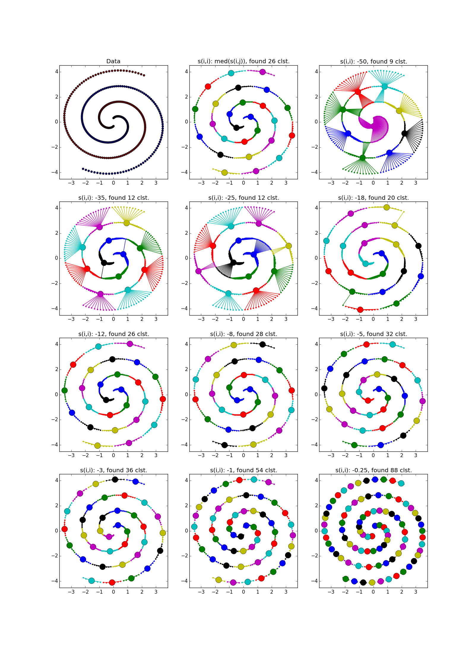
Если складка пересекает другой сгусток, дело обстоит хуже, но даже так AP помогает понять, что в этом месте творится что-то интересное.
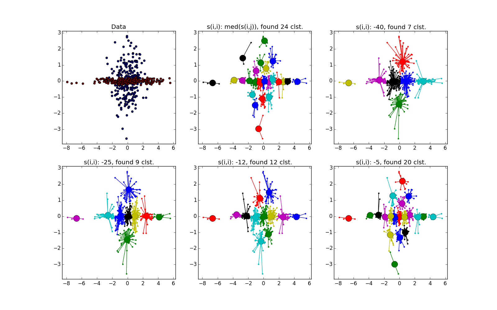
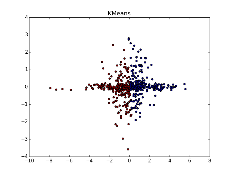
При хорошем подборе параметра и кластеризатора-постобработчика AP выигрывает и в случае кластеров разного размера. Обратите внимание на картинку с - almost perfect partition, if you combine clusters from top to right.
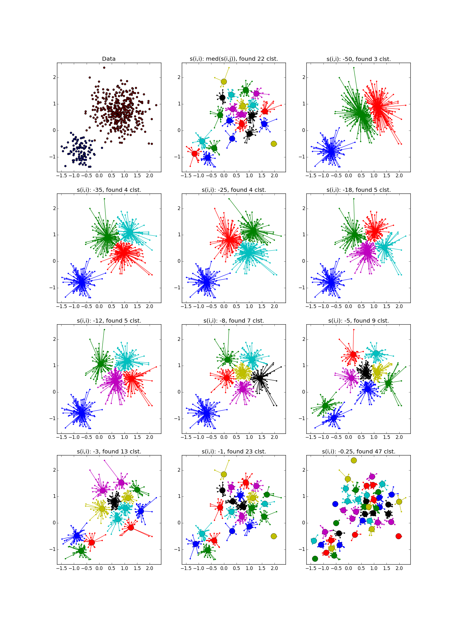
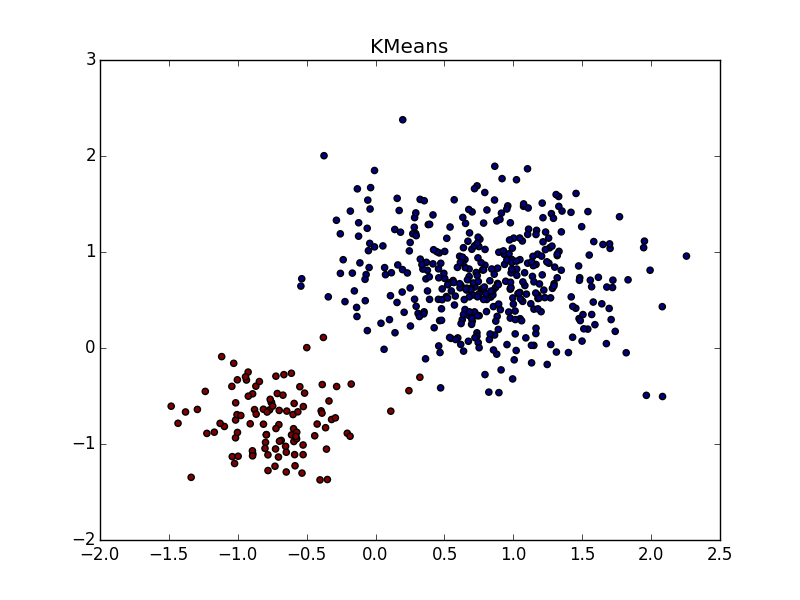
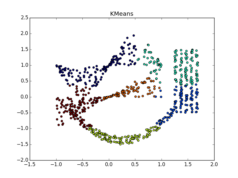
With clusters of the same shape, but with different densities, AP and k-means plus or minus parity. In one case, you need to guess right and in another - .


With a bunch of higher density in another bunch, in my opinion, k-means wins a little. He, of course, “eats away” a significant chunk in favor of a cluster of higher density, but according to the visual result of the AP's work, heterogeneity is not very visible at all.
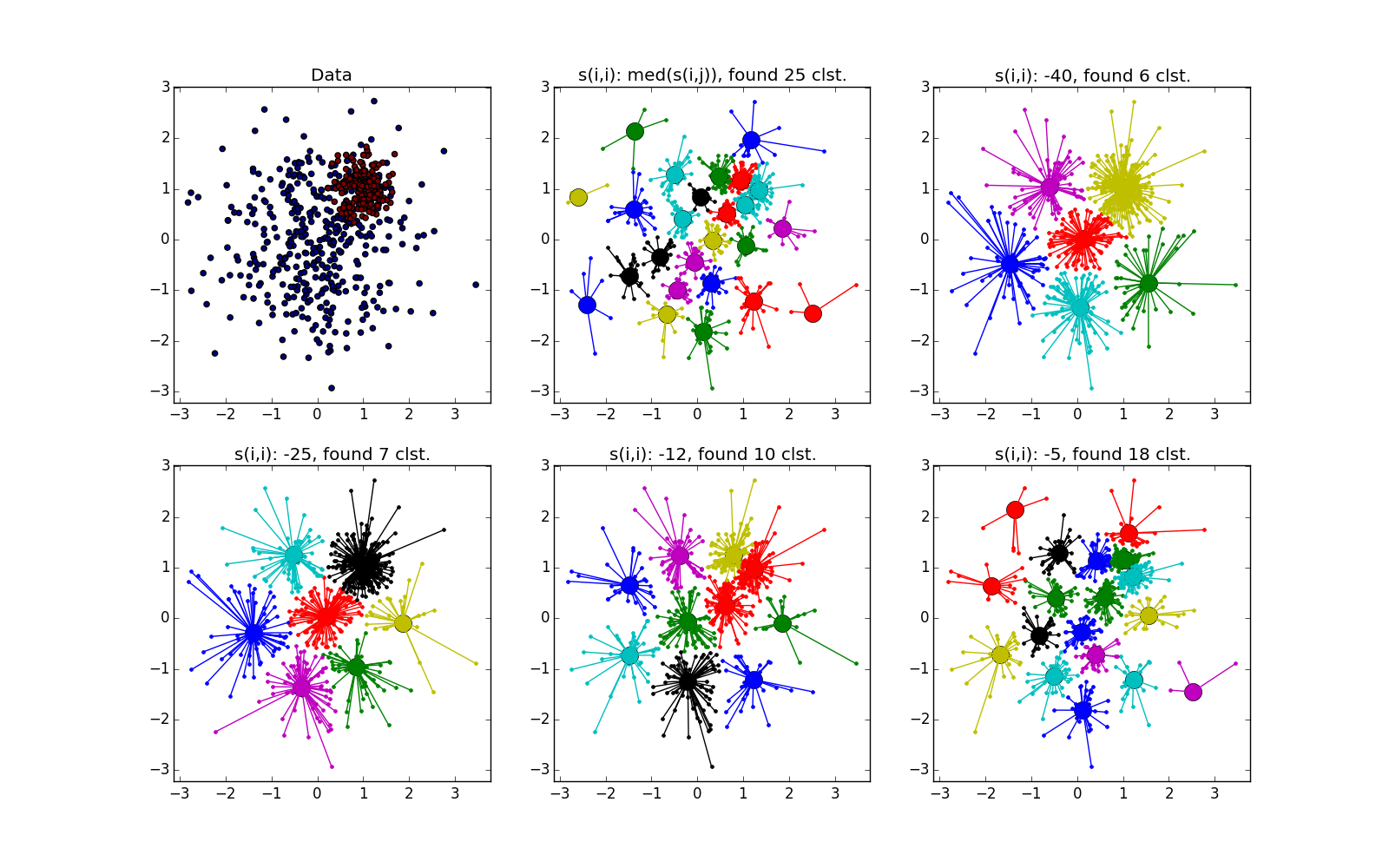
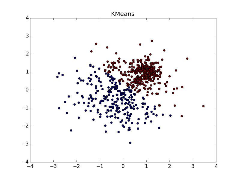
A few more pictures:
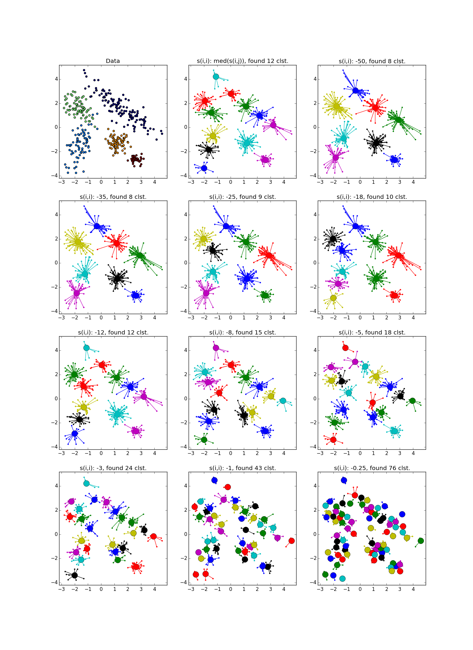
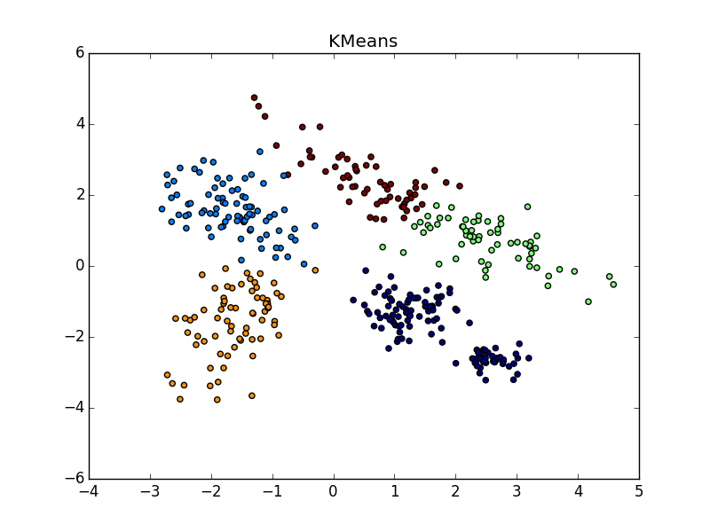
Если складка пересекает другой сгусток, дело обстоит хуже, но даже так AP помогает понять, что в этом месте творится что-то интересное.
При хорошем подборе параметра и кластеризатора-постобработчика AP выигрывает и в случае кластеров разного размера. Обратите внимание на картинку с
- almost perfect partition, if you combine clusters from top to right. With clusters of the same shape, but with different densities, AP and k-means plus or minus parity. In one case, you need to guess right
and in another - . With a bunch of higher density in another bunch, in my opinion, k-means wins a little. He, of course, “eats away” a significant chunk in favor of a cluster of higher density, but according to the visual result of the AP's work, heterogeneity is not very visible at all.
A few more pictures:
Total
Use affinity propagation when
- You are not very big (
 ) or moderately large, but sparse (
 ) dataset
 - Proximity function known in advance
- You expect to see many clusters of various shapes and slightly varying numbers of elements.
- Are you ready to tinker with post-processing
- The complexity of the dataset elements does not matter
- Properties of the proximity function do not matter
- The number of clusters does not matter
Allegedly , various scientists have successfully used affinity propagation to
- Image segmentation
- Isolation of groups in the genome
- Partitioning cities by accessibility
- Clustering Granite Samples
- Movie Grouping on Netflix
In all these cases, the result was better than with k-means. Not that it’s some kind of super result in itself. I do not know whether in all these cases a comparison was made with other algorithms. I plan to do this in future articles. Apparently, on datasets from real life, the ability to spread proximity to deal with clusters of different geometric shapes helps the most.
Well, that’s all. Next time, consider another algorithm and compare it with the proximity propagation method. Good luck, Habr!