Procedural vegetation on OpenGL and GLSL
In this post I would like to talk about using hardware tessellation and a geometric shader to generate a large amount of geometry based on minimal input. I hope the post will be useful to those who have an initial understanding of shader programming, but have not yet realized the full power of a programmable graphics pipeline. This is not a guide for shaders for beginners, so many aspects of their work are visible under the carpet or provided with a link to the relevant documentation.

The narration will be conducted on the example of a small demo that generates a scene like in the picture above. We will go through an exciting journey from preparing data on the CPU to writing color values to the output of the fragment shader.
When writing the demo, I set the following goals:
Based on this list, I had to sacrifice the study of some points:
In order to provide the reader with the opportunity to review the entire code of the demo during the course of the story, I will immediately give a link to the repository.
We will draw a set of patches , each of which contains a single vertex. Each vertex, in turn, contains a single four-component attribute. Using this minimal portion of data as a seed, we will “grow” on each such patch (ie, one point) a whole bush of moving stems. In addition, all bushes can be exposed to wind with user-defined parameters. Most of the bush generation work is done in the Tesselation evaluation shader and in the geometric shader. So, in the tessellation shader, a bush skeleton is generated with all the deformations introduced by stirring and wind, and in the geometric shader, a polygonal “flesh” is stretched onto this skeleton, the thickness of which depends on the height of the bone on the skeleton. The fragment shader, as usual, calculates the lighting and applies a procedurally generated texture based on the Voronoi diagram.
So, let's begin!
The way of data to colorize the monitor pixels begins with their preparation on the CPU. As mentioned above, each "model" of the scene initially consists of one vertex. Let's make this vertex four-dimensional, where the first three components are the position of the vertex in space, and the fourth component is the number of stems in the bush. Thus, the bushes will be able to differ from each other in the number of stems. We begin the generation of coordinates from nodes of a square lattice of finite size, and we perturb each coordinate by a random value from a given interval:
We will send the generated data to the video memory:
Now the method of rendering the entire lawn from the generated grass looks very concise:
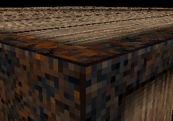
In addition to geometry, in shaders we need evenly distributed random numbers. It is most optimal to get numbers in the interval [0; 1], and on the GPU in each particular place bring them to the required interval. We will deliver them to the video memory in the form of a one-dimensional texture, for which the closest value is set as the filtering. Let me remind you that in the two-dimensional case, such filtering leads to a similar result:
Source
Code for generating and adjusting the texture:
As a rule, when using tessellation, the vertex shader turns out to be very lazy, since the pipeline starts from it, and there is no geometry as such yet. In our case, the vertex shader is trivial. In it, we simply send a point from the entrance immediately to the exit:
Hardware tessellation is a powerful technique for increasing the granularity of polygonal models using GPUs. Do not confuse with the algorithms for splitting polygons into triangles performed on the central processor. Hardware tessellation consists of three stages of the graphics pipeline, two of which can be programmed (highlighted in yellow):

More details about shaders and their inputs / outputs are described below. Here it is worth saying that a patch consisting of an arbitrary number of vertices is applied to the tessellation input, which is fixed for each glDraw * call and is limited to at least 32. The attributes of these vertices do not have any highlighted values, which means that the programmer is free to interpret them in both shaders as you wish. This provides truly fantastic opportunities compared to the old vertex shaders.
The model of work of programmable tessellation differs significantly from other shaders, and can be bewildering when you first get acquainted with it, even if you have experience working with vertex and geometric shaders.
In the general case, all vertices of the input patch that have passed through the vertex shader separately are available to the tessellation control shader. It receives the number of vertices in the gl_PatchVerticesIn patch, the sequence number of the gl_PrimitiveID patch, and the serial number of the output vertex gl_InvocationID, which will be discussed later. The sequence number of the gl_PrimitiveID patch counts as part of a single glDraw * call. The vertex data itself is accessible through an array of gl_in structures, declared as follows:
This array is indexed from zero to gl_PatchVerticesIn - 1. Of greatest interest in this declaration is the gl_Position field, which contains data from the output of the vertex shader. The number of vertices of the output patch is set in the code of the shader by the global declaration:
and it does not have to match the number of vertices in the input patch. The number of shader calls is equal to the number of output vertices. In each call, the shader has access to all the input vertices of the patch, but it can write only on the index gl_InvocationID of the output array gl_out, which is declared as
Now let's move on to a more interesting fact. The shader can only write by gl_InvocationID, however it can read the outputarray at any index! We remember that the work of shaders is very much parallelized, and the order of their call is not deterministic. This imposes restrictions on the sharing of data by shaders, but makes SIMD-parallelism possible and gives the compiler carte blanche to use the most severe optimizations. To prevent these rules from being violated, barrier synchronization is available in the tessellation control shader. Calling the built-in barrier () function blocks execution until all patch shaders invoke this function. Serious restrictions are imposed on the call to this function: it cannot be called from any function except main, it cannot be called in any flow control construct (for, while, switch), and it cannot be called after return.
And finally, the most interesting thing at this stage of the pipeline: the output of the vertices is not the main thing. Polygons will not be collected from the coordinates recorded in gl_out. The main product of the tessellation control shader is writing to the following output arrays:
These arrays control the number of vertices in the so-called abstract patches , and that is why this stage is called tessellation control. An abstract patch is a set of points of a two-dimensional geometric shape that is generated at the tessellation primitive generation stage. Abstract patches come in three forms: triangles, squares, and contours. In this case, for each type of abstract patch, the shader should fill in only the indices gl_TessLevelOuter and gl_TessLevelInner it needs, and the remaining indices of these arrays are ignored. The generated patch contains not only the vertices of the geometric figure, but also the coordinates of the points on the borders and inside the figure. For example, a square with some values of gl_TessLevelOuter and gl_TessLevelInner will be formed from triangles of this kind:
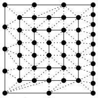
The lower left corner of the square always has the coordinate [0; 0], the upper right - [1; 1], and all other points will have corresponding coordinates with values from 0 to 1.
Isolines are essentially a square, divided into rectangles, and not into triangles. The values of the coordinates of the points on the contours will also belong to the interval from 0 to 1.
But the coordinates inside the triangle are fundamentally different: in a two-dimensional triangle, three-component barycentric coordinates are used . Moreover, their values also lie in the interval from 0 to 1, and the triangle is equilateral.
The specific type of partition (which, in fact, is called tessellation in the original sense) of an abstract patch depends heavily on gl_TessLevelOuter and gl_TessLevelInner. We will not dwell on it here in detail, nor will we analyze how Inner differs from Outer. All this is described in detail in the corresponding section of the OpenGL manual.
Now back to our plants. At this stage of the graphics pipeline, we still cannot perform any meaningful transformations on the existing single point, therefore we will give the input vertex to the output of this shader without changes:
To generate the geometry, we will use a rectangular lattice, that is, an abstract patch of the "isoline" type. Isoline generation is controlled by only two variables: gl_TessLevelOuter [0] - the number of points along the y coordinate , and gl_TessLevelOuter [1] - the number of points along the x . In our program, a cycle along y will run through the stems of the bush, and for each stem a cycle along x will run along the stem. Therefore, we record the number of stems (the fourth coordinate of the input point) on the corresponding output:
The number of points along the stem determines the number of segments of which the stem is composed, that is, its detail. In order not to waste resources, we will make the level of detail dependent on the distance between the camera and the bush:
On the CPU side, homogeneous variables are populated before each glDraw * call:
The first of them is the coordinates of the camera in space, and the second is the direction of view. Knowing the position of the camera, the direction of view and the coordinate of the bush, we can find out if this bush is behind the camera:
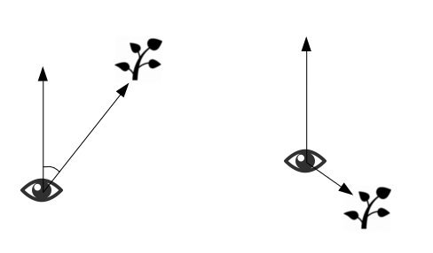
If the bush is in front, then the angle between the direction from the camera forward and from the camera to the bush will be sharp, otherwise it will be dull. Accordingly, in the first case, the scalar product of the vectors shown in the figure will be greater than zero, and in the second, less. We calculate the scalar product and use the step function with a step at zero to get a variable that is zero if the bush is behind and one if it is in front:
Finally, we can record the number of points for the stems of the future bush:
A note on terminology: in the English original, this shader is called the Tesselation evaluation shader . On the Russian Internet, you can find literal translations like “tessellation evaluation shader” or “tessellation calculation shader”. They look awkward and, in my opinion, do not reflect the essence of this shader. Therefore, here the tesselation evaluation shader will be called simply the tessellation shader, unlike the previous stage, where the tessellation control shader was.
Tessellation is enabled only if the tessellation shader is added to the shader program. At the same time, the tessellation control shader is not mandatory: its absence is equivalent to applying the input patch to the output without changes. The values of the gl_TessLevel * arrays can be set on the CPU side by calling glPatchParameterfv with the parameter GL_PATCH_DEFAULT_OUTER_LEVEL or GL_PATCH_DEFAULT_INNER_LEVEL. In this case, all abstract patches in the tessellation shader will be the same. Adding only a tessellation control shader to the program does not make sense and leads to a shader layout error. The appearance of the abstract patch, in contrast to its parameters, is determined in the tessellation shader code:
The tessellation shader is invoked for each point in the abstract patch. For example, if we ordered contours with dots 64x64, then the shader will be called 4096 times. All peaks from the output of the tessellation control shader come to its input:
as well as gl_PatchVerticesIn, gl_PrimitiveID, gl_TessLevelOuter, and gl_TessLevelInner already familiar to us. The last two variables are of the same type as in the tessellation control shader, but are read-only. Finally, the most interesting input variable is
It contains the coordinates of the current (for this call) point of the abstract patch. It is declared as vec3, however gl_TessCoord.z only makes sense for triangles. The reading of this coordinate for squares or contours is not defined.
Several variables can be applied to the output of the shader. The main one is vec4 gl_Position, in which you need to record the coordinates of the vertices from which primitives will be collected for the next stage of the pipeline. In our case, this is a sequence of segments, because the tessellation shader produces only the skeleton for the future bush.
So, we have many (up to 4096) vertices of the abstract patch, organized in lines that are divided into equal segments. If we draw this shape as lines without changes:
we’ll see something similar to the pictures in the documentation :
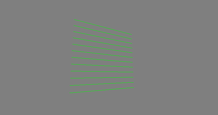
Hereinafter in the screenshots, a little side view
How to make stems from these lines? To start, put them vertically:

and learn how to arrange them in a circle, turning around a vertical axis:
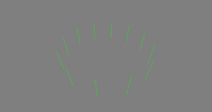
However, such lines look more like a fence than a bush. To make our bush more natural, let's bend the line like a cubic Bezier curve:

And here the coordinate gl_TessCoord.x is very useful, about which we agreed to think that it runs along each stem from zero to one. The form of the curve completely depends on the reference points P 0 ... P 3 . The bottom of the stem will always be located on the ground, and its top should always look towards the sky, so we take P 0 = (0; 0). And to select at least the approximate position of the remaining free points, cubic-bezier.com is perfectwhose sole purpose is to construct a curve of the required form. Now if we substitute gl_TessCoord.x into the formula of the Bezier curve, we get a polyline, the vertices of which lie on the curve, and the segments approximate the curve:
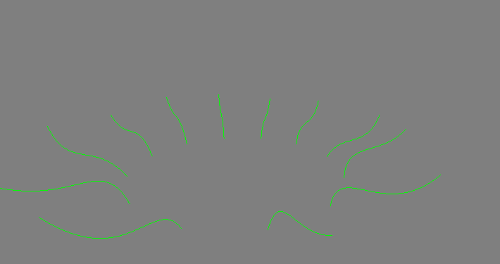
In the future, we will need to build up polygons around a curved stem, for which at each vertex of the broken stem we need to know a plane perpendicular to the stem. From the course of differential geometry it is known that the vector of the main normal to the parametric curve can be obtained as a combination of vector products of the derivatives of the curve with respect to the parameter:
[B ', [B', B '']] (1)
To uniquely specify a plane, we need one more vector. In our case, the entire curve is located in the vertical plane XY, which means that the main normal to is located in it. Therefore, the binormal to the curve is given to us for free - it is just a constant vector (0; 0; 1). Now we recall that from a cozy XY plane, the stem rotates around the origin, which means that the normal plane must also be rotated. To do this, it is enough to multiply both of its generating vectors by the same rotation matrix as the points of the stem. Putting it all together:
And for clarity, we reduce the detail of the stems. The normals are drawn in red, and the binormals are drawn in blue:

Now, briefly about the animation. First, the stems move by themselves. This is done through the circular rotation of the anchor points of the curve around other, original points. The position of the initial points and the initial phase of rotation depend on a random variable (remember the random one-dimensional texture?), Which, in turn, depends on gl_TessCoord.y and gl_PrimitiveID. Thus, each stem in each bush moves in its own way, which creates the illusion of chaos. And since the movement is done through the movement of control points, the normals and binormals remain completely correct. In fact, we got a skeletal animation, in which bones are generated on the fly, and do not occupy memory.
In addition to their own movement of the bushes, they are still affected by the "wind". Wind is the displacement of the vertices of the stem in the direction specified by the user by an amount that depends on two user parameters and Perlin noise. In this case, the wind should not displace the roots of the stems, therefore, the amount of displacement is multiplied by the flexibility function:
taken from the coordinate along the stem t1. Custom wind parameters are called “speed” and “turbulence” purely conditionally, because changing them in the range accessible to the user is similar to changing these air flow parameters. However, this “wind” has nothing to do with real physics. The speed slider in the interface is intentionally limited to a small amount, because the wind is applied to the skeleton after calculating the normals without adjusting them. Because of this, the normals cease to be such, and with a strong skeleton distortion (large "wind speed"), self-intersections of polygons appear.
Why is Perlin noise if there is a “noisy” texture? The fact is that texture values are not a continuous function of the coordinate, in contrast to Perlin noise. Therefore, if we make an offset depending on the noisy texture in each frame, we get chaotic twitching with a frame rate instead of a smooth wind. The high-quality implementation of Perlin's noise was taken from Stefan Gustavson .
What else will be needed to build polygons? First, the thickness of the stem should decrease from the root to the apex. Therefore, we will create the corresponding output variable and pass the thickness into it, depending on the coordinate along the stem:
The coordinate along the stem and the number of the stem in the bush will also be transferred further along the conveyor:
We will need them when applying texture.
Finally we came to the completion of the geometric part of our path. At the input of the geometric shader, we get the whole primitives. If at the input of the tessellation stage there were arbitrary patches that could contain a decent amount of data, then here the primitives are points, lines, or triangles. If there are no tessellation shaders, then primitives (usually triangles) from the glDraw * call appear on the input of the geometric shader, which may have been vertically processed by the vertex shader. In our case, tessellation produces contours that we accept as segments, that is, pairs of vertices:
These vertices are written to the built-in input array.
which in our case can be indexed only by zero or by one. User input variables are also defined as arrays with the same range of indices:
The output of the geometric shader can be fed points, a sequence of lines or a sequence of triangles. We will use the last option:
A shader is called for each input primitive and can produce several primitives. This is done using two built-in functions. As in the previous stages, the output variable is called gl_Position. After filling it, the shader should call the built-in function EmitVertex () to inform the video card about the end of the vertex formation. At the end of the formation of all vertices of the primitive, the EndPrimitive () function is called;
The polygons of the stem are formed simply: knowing the planes perpendicular to the curve of the stem at the beginning and at the end of the segment, we move in these planes around the point of intersection with the segment and release the vertices with some step. The detail depends on this step, i.e. whether the stem will look more like a pyramid or a cone.
For example, this is how a bush of 5-sector stems looks like with non-interpolated (flat) coordinates and fragment normals for clarity:
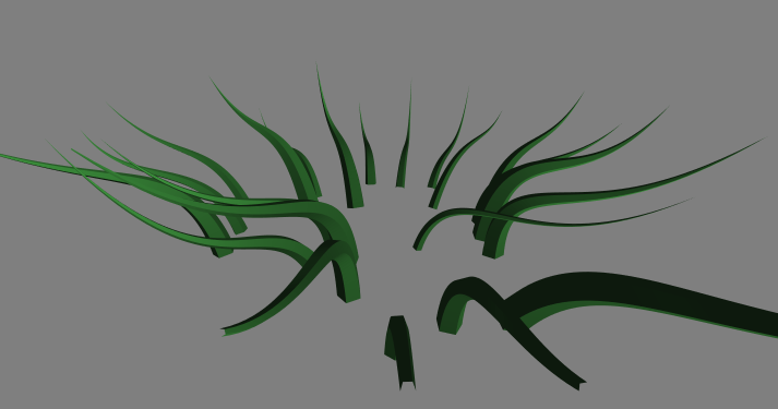
And here is a code that implements the described approach:
The fragment shader looks pretty standard, so I'll talk about it briefly. In it, the usual Fong lighting is summarized with the procedural texture in the form of cells based on the Voronoi diagram, taken from Stephen Gustavson, already familiar to us. The color of the texel depends not only on the texture coordinates, but also on time (frame number) and on the number of the stem in the bush:
Thus, the cells smoothly “creep” along the stem, looking different on different stems.
This ends the data path along the graphics pipeline, which means it's time to take stock.
So, what have we won in comparison with more traditional approaches? Answer: memory, flexibility and bandwidth savings. When trying to make an animation of similar flexibility in another way, we would have to do some of this:
Most of the links are already in the text. Here I would like to leave useful links that were used during the work on the demo:
Thanks for attention!
UPD1
UPD2
Link to binaries for Windows.
The narration will be conducted on the example of a small demo that generates a scene like in the picture above. We will go through an exciting journey from preparing data on the CPU to writing color values to the output of the fragment shader.
Goals and means
When writing the demo, I set the following goals:
- Minimize the amount of data stored in video memory. Consequently:
- Dispose of the GPU as much as possible using all the available stages of the pipeline.
- Make some scene settings customizable.
- Focus on geometry and writing shaders, spending a minimum of effort on the rest of the components. Therefore, the most familiar instrumentation was used: C ++ 11 (gcc), Qt5 + qmake, GLSL.
- If possible, simplify the assembly and launch of the resulting demo on various platforms.
Based on this list, I had to sacrifice the study of some points:
- The main loop is made primitively. Therefore, the speed of animation and movement of the camera depends on the frame rate, and therefore on the position of the camera in space.
- In a single class of the camera its coordinates, orientation, projection and functions are involved to change all this. In this form, writing it did not take much time and allowed us to make a fairly optimal forward of the camera parameters into the shader.
- The shader class is made in the form of a fairly thin wrapper over the corresponding Qt5 class. The pieces of code that are common for different stages are glued together and given to the compiler optimizer, which will throw out unused code and global variables.
- The program uses a single shader, so the data transfer to it is done without the "newfangled" UBO . In this case, they would not add performance by complicating the code.
- The frame per second counter is based on OpenGL queries . Therefore, it does not show “real” FPS, but a slightly overestimated idealized indicator, which does not take into account the overhead introduced by Qt.
- Cool lighting was not the goal of writing this demo, so a simple implementation of Phong lighting with one light source in the shader is used.
- The implementation of noise in the shaders was taken from a third-party author.
In order to provide the reader with the opportunity to review the entire code of the demo during the course of the story, I will immediately give a link to the repository.
A brief overview of geometry generation
We will draw a set of patches , each of which contains a single vertex. Each vertex, in turn, contains a single four-component attribute. Using this minimal portion of data as a seed, we will “grow” on each such patch (ie, one point) a whole bush of moving stems. In addition, all bushes can be exposed to wind with user-defined parameters. Most of the bush generation work is done in the Tesselation evaluation shader and in the geometric shader. So, in the tessellation shader, a bush skeleton is generated with all the deformations introduced by stirring and wind, and in the geometric shader, a polygonal “flesh” is stretched onto this skeleton, the thickness of which depends on the height of the bone on the skeleton. The fragment shader, as usual, calculates the lighting and applies a procedurally generated texture based on the Voronoi diagram.
So, let's begin!
CPU
The way of data to colorize the monitor pixels begins with their preparation on the CPU. As mentioned above, each "model" of the scene initially consists of one vertex. Let's make this vertex four-dimensional, where the first three components are the position of the vertex in space, and the fourth component is the number of stems in the bush. Thus, the bushes will be able to differ from each other in the number of stems. We begin the generation of coordinates from nodes of a square lattice of finite size, and we perturb each coordinate by a random value from a given interval:
const int numNodes = 14; // Количество узлов решётки вдоль одной стороны.
const GLfloat gridStep = 3.0f; // Шаг решётки.
// Максимальные смещения в горизонтальной плоскости:
const GLfloat xDispAmp = 5.0f;
const GLfloat zDispAmp = 5.0f;
const GLfloat yDispAmp = 0.3f; // Максимальное смещение по вертикали.
numClusters = numNodes * numNodes; // Количество кустов.
GLfloat *vertices = new GLfloat[numClusters * 4]; // Буфер для генерируемых вершин.
std::random_device rd;
std::mt19937 mt(rd());
std::uniform_real_distribution xDisp(-xDispAmp, xDispAmp);
std::uniform_real_distribution yDisp(-yDispAmp, yDispAmp);
std::uniform_real_distribution zDisp(-zDispAmp, zDispAmp);
std::uniform_int_distribution numStems(12, 64); // Количество стеблей.
for(int i = 0; i < numNodes; ++i) {
    for(int j = 0; j < numNodes; ++j) {
	const int idx = (i * numNodes + j) * 4;
	vertices[idx]     = (i - numNodes / 2) * gridStep + xDisp(mt);
	vertices[idx + 1] = yDisp(mt);
	vertices[idx + 2] = (j - numNodes / 2) * gridStep + zDisp(mt);
	vertices[idx + 3] = numStems(mt);
    }
}
We will send the generated data to the video memory:
GLuint vao; // https://www.opengl.org/wiki/Vertex_Specification#Vertex_Array_Object
GLuint posVbo; // https://www.opengl.org/wiki/Vertex_Specification#Vertex_Buffer_Object
glGenVertexArrays(1, &vao);
glBindVertexArray(vao);
glGenBuffers(1, &posVbo);
glEnableVertexAttribArray(ATTRIBINDEX_VERTEX);
glBindBuffer(GL_ARRAY_BUFFER, posVbo);
glVertexAttribPointer(ATTRIBINDEX_VERTEX, 4, GL_FLOAT, GL_FALSE, 0, 0);
glBufferData(GL_ARRAY_BUFFER, sizeof(GLfloat) * numClusters * 4, vertices, GL_STATIC_DRAW);
glFinish();
delete[] vertices;
Now the method of rendering the entire lawn from the generated grass looks very concise:
void ProceduralGrass::draw() {
    glBindVertexArray(vao);
    glPatchParameteri(GL_PATCH_VERTICES, 1);
    glDrawArrays(GL_PATCHES, 0, numClusters);
    glBindVertexArray(0);
}
In addition to geometry, in shaders we need evenly distributed random numbers. It is most optimal to get numbers in the interval [0; 1], and on the GPU in each particular place bring them to the required interval. We will deliver them to the video memory in the form of a one-dimensional texture, for which the closest value is set as the filtering. Let me remind you that in the two-dimensional case, such filtering leads to a similar result:
Source
Code for generating and adjusting the texture:
const GLuint randTexSize = 256;
GLfloat randTexData[randTexSize];
std::random_device rd;
std::mt19937 gen(rd());
std::uniform_real_distribution dis(0.0f, 1.0f);
std::generate(randTexData, randTexData + randTexSize, [&](){return dis(gen);});
// Create and tune random texture.
glGenTextures(1, &randTexture);
glActiveTexture(GL_TEXTURE0);
glBindTexture(GL_TEXTURE_1D, randTexture);
glTexParameteri(GL_TEXTURE_1D, GL_TEXTURE_MIN_FILTER, GL_NEAREST);
glTexParameteri(GL_TEXTURE_1D, GL_TEXTURE_MAG_FILTER, GL_NEAREST);
glTexParameteri(GL_TEXTURE_1D, GL_TEXTURE_WRAP_S, GL_REPEAT);
glTexParameteri(GL_TEXTURE_1D, GL_TEXTURE_BASE_LEVEL, 0);
glTexParameteri(GL_TEXTURE_1D, GL_TEXTURE_MAX_LEVEL, 0);
glTexImage1D(GL_TEXTURE_1D, 0, GL_R16F, randTexSize, 0, GL_RED, GL_FLOAT, randTexData);
glUniform1i(glGetUniformLocation(grassShader.programId(), "urandom01"), 0);
Vertex shader
As a rule, when using tessellation, the vertex shader turns out to be very lazy, since the pipeline starts from it, and there is no geometry as such yet. In our case, the vertex shader is trivial. In it, we simply send a point from the entrance immediately to the exit:
layout(location=0) in vec4 position;
void main(void) {
    gl_Position = position;
}
Tessellation
Hardware tessellation is a powerful technique for increasing the granularity of polygonal models using GPUs. Do not confuse with the algorithms for splitting polygons into triangles performed on the central processor. Hardware tessellation consists of three stages of the graphics pipeline, two of which can be programmed (highlighted in yellow):
More details about shaders and their inputs / outputs are described below. Here it is worth saying that a patch consisting of an arbitrary number of vertices is applied to the tessellation input, which is fixed for each glDraw * call and is limited to at least 32. The attributes of these vertices do not have any highlighted values, which means that the programmer is free to interpret them in both shaders as you wish. This provides truly fantastic opportunities compared to the old vertex shaders.
The model of work of programmable tessellation differs significantly from other shaders, and can be bewildering when you first get acquainted with it, even if you have experience working with vertex and geometric shaders.
Tessellation control shader
In the general case, all vertices of the input patch that have passed through the vertex shader separately are available to the tessellation control shader. It receives the number of vertices in the gl_PatchVerticesIn patch, the sequence number of the gl_PrimitiveID patch, and the serial number of the output vertex gl_InvocationID, which will be discussed later. The sequence number of the gl_PrimitiveID patch counts as part of a single glDraw * call. The vertex data itself is accessible through an array of gl_in structures, declared as follows:
in gl_PerVertex
{
  vec4 gl_Position;
  float gl_PointSize;
  float gl_ClipDistance[];
} gl_in[gl_MaxPatchVertices];
This array is indexed from zero to gl_PatchVerticesIn - 1. Of greatest interest in this declaration is the gl_Position field, which contains data from the output of the vertex shader. The number of vertices of the output patch is set in the code of the shader by the global declaration:
layout (vertices = 1) out; // В данном случае задана одна вершина
and it does not have to match the number of vertices in the input patch. The number of shader calls is equal to the number of output vertices. In each call, the shader has access to all the input vertices of the patch, but it can write only on the index gl_InvocationID of the output array gl_out, which is declared as
out gl_PerVertex
{
  vec4 gl_Position;
  float gl_PointSize;
  float gl_ClipDistance[];
} gl_out[];
Now let's move on to a more interesting fact. The shader can only write by gl_InvocationID, however it can read the outputarray at any index! We remember that the work of shaders is very much parallelized, and the order of their call is not deterministic. This imposes restrictions on the sharing of data by shaders, but makes SIMD-parallelism possible and gives the compiler carte blanche to use the most severe optimizations. To prevent these rules from being violated, barrier synchronization is available in the tessellation control shader. Calling the built-in barrier () function blocks execution until all patch shaders invoke this function. Serious restrictions are imposed on the call to this function: it cannot be called from any function except main, it cannot be called in any flow control construct (for, while, switch), and it cannot be called after return.
And finally, the most interesting thing at this stage of the pipeline: the output of the vertices is not the main thing. Polygons will not be collected from the coordinates recorded in gl_out. The main product of the tessellation control shader is writing to the following output arrays:
patch out float gl_TessLevelOuter[4];
patch out float gl_TessLevelInner[2];
These arrays control the number of vertices in the so-called abstract patches , and that is why this stage is called tessellation control. An abstract patch is a set of points of a two-dimensional geometric shape that is generated at the tessellation primitive generation stage. Abstract patches come in three forms: triangles, squares, and contours. In this case, for each type of abstract patch, the shader should fill in only the indices gl_TessLevelOuter and gl_TessLevelInner it needs, and the remaining indices of these arrays are ignored. The generated patch contains not only the vertices of the geometric figure, but also the coordinates of the points on the borders and inside the figure. For example, a square with some values of gl_TessLevelOuter and gl_TessLevelInner will be formed from triangles of this kind:
The lower left corner of the square always has the coordinate [0; 0], the upper right - [1; 1], and all other points will have corresponding coordinates with values from 0 to 1.
Isolines are essentially a square, divided into rectangles, and not into triangles. The values of the coordinates of the points on the contours will also belong to the interval from 0 to 1.
But the coordinates inside the triangle are fundamentally different: in a two-dimensional triangle, three-component barycentric coordinates are used . Moreover, their values also lie in the interval from 0 to 1, and the triangle is equilateral.
The specific type of partition (which, in fact, is called tessellation in the original sense) of an abstract patch depends heavily on gl_TessLevelOuter and gl_TessLevelInner. We will not dwell on it here in detail, nor will we analyze how Inner differs from Outer. All this is described in detail in the corresponding section of the OpenGL manual.
Now back to our plants. At this stage of the graphics pipeline, we still cannot perform any meaningful transformations on the existing single point, therefore we will give the input vertex to the output of this shader without changes:
gl_out[gl_InvocationID].gl_Position = gl_in[gl_InvocationID].gl_Position;
To generate the geometry, we will use a rectangular lattice, that is, an abstract patch of the "isoline" type. Isoline generation is controlled by only two variables: gl_TessLevelOuter [0] - the number of points along the y coordinate , and gl_TessLevelOuter [1] - the number of points along the x . In our program, a cycle along y will run through the stems of the bush, and for each stem a cycle along x will run along the stem. Therefore, we record the number of stems (the fourth coordinate of the input point) on the corresponding output:
gl_TessLevelOuter[0] = gl_in[gl_InvocationID].gl_Position.w;
The number of points along the stem determines the number of segments of which the stem is composed, that is, its detail. In order not to waste resources, we will make the level of detail dependent on the distance between the camera and the bush:
uniform vec3 eyePosition; // Положение камеры передаётся в эту переменную из объекта камеры.
int lod() {
    // Расстояние от камеры до куста:
    float dist = distance(gl_in[gl_InvocationID].gl_Position.xyz, eyePosition);
    // Количество точек на стебле в зависимости от расстояния:
    if(dist < 10.0f) {
        return 48;
    }
    if(dist < 20.0f) {
        return 24;
    }
    if(dist < 80.0f) {
        return 12;
    }
    if(dist < 800.0f) {
        return 6;
    }
    return 4;
}
On the CPU side, homogeneous variables are populated before each glDraw * call:
grassShader.setUniformValue("eyePosition", camera.getPosition());
grassShader.setUniformValue("lookDirection", camera.getLookDirection());
The first of them is the coordinates of the camera in space, and the second is the direction of view. Knowing the position of the camera, the direction of view and the coordinate of the bush, we can find out if this bush is behind the camera:
If the bush is in front, then the angle between the direction from the camera forward and from the camera to the bush will be sharp, otherwise it will be dull. Accordingly, in the first case, the scalar product of the vectors shown in the figure will be greater than zero, and in the second, less. We calculate the scalar product and use the step function with a step at zero to get a variable that is zero if the bush is behind and one if it is in front:
float halfspaceCull = step(dot(eyePosition - gl_in[gl_InvocationID].gl_Position.xyz, lookDirection), 0);
Finally, we can record the number of points for the stems of the future bush:
gl_TessLevelOuter[1] = lod() * halfspaceCull;
Tessellation shader
A note on terminology: in the English original, this shader is called the Tesselation evaluation shader . On the Russian Internet, you can find literal translations like “tessellation evaluation shader” or “tessellation calculation shader”. They look awkward and, in my opinion, do not reflect the essence of this shader. Therefore, here the tesselation evaluation shader will be called simply the tessellation shader, unlike the previous stage, where the tessellation control shader was.
Tessellation is enabled only if the tessellation shader is added to the shader program. At the same time, the tessellation control shader is not mandatory: its absence is equivalent to applying the input patch to the output without changes. The values of the gl_TessLevel * arrays can be set on the CPU side by calling glPatchParameterfv with the parameter GL_PATCH_DEFAULT_OUTER_LEVEL or GL_PATCH_DEFAULT_INNER_LEVEL. In this case, all abstract patches in the tessellation shader will be the same. Adding only a tessellation control shader to the program does not make sense and leads to a shader layout error. The appearance of the abstract patch, in contrast to its parameters, is determined in the tessellation shader code:
layout(isolines, equal_spacing) in; // В нашем случае это изолинии.
The tessellation shader is invoked for each point in the abstract patch. For example, if we ordered contours with dots 64x64, then the shader will be called 4096 times. All peaks from the output of the tessellation control shader come to its input:
in gl_PerVertex
{
  vec4 gl_Position;
  float gl_PointSize;
  float gl_ClipDistance[];
} gl_in[gl_MaxPatchVertices];
as well as gl_PatchVerticesIn, gl_PrimitiveID, gl_TessLevelOuter, and gl_TessLevelInner already familiar to us. The last two variables are of the same type as in the tessellation control shader, but are read-only. Finally, the most interesting input variable is
in vec3 gl_TessCoord;
It contains the coordinates of the current (for this call) point of the abstract patch. It is declared as vec3, however gl_TessCoord.z only makes sense for triangles. The reading of this coordinate for squares or contours is not defined.
Several variables can be applied to the output of the shader. The main one is vec4 gl_Position, in which you need to record the coordinates of the vertices from which primitives will be collected for the next stage of the pipeline. In our case, this is a sequence of segments, because the tessellation shader produces only the skeleton for the future bush.
So, we have many (up to 4096) vertices of the abstract patch, organized in lines that are divided into equal segments. If we draw this shape as lines without changes:
gl_Position = vec4(gl_TessCoord.xy, 0.0f, 1.0f);
we’ll see something similar to the pictures in the documentation :
Hereinafter in the screenshots, a little side view
How to make stems from these lines? To start, put them vertically:
gl_Position = vec4(gl_TessCoord.yx, 0.0f, 1.0f);
and learn how to arrange them in a circle, turning around a vertical axis:
vec3 position = vec3(2.0f, gl_TessCoord.x, 0.0f);
float alpha = gl_TessCoord.y * 2.0f * M_PI;
float cosAlpha = cos(alpha);
float sinAlpha = sin(alpha);
mat3 circDistribution = mat3(
    cosAlpha, 0.0f, -sinAlpha,
    0.0f,     1.0f,      0.0f,
    sinAlpha, 0.0f, cosAlpha);
position = circDistribution * position;
gl_Position = vec4(position, 1.0f);
However, such lines look more like a fence than a bush. To make our bush more natural, let's bend the line like a cubic Bezier curve:
And here the coordinate gl_TessCoord.x is very useful, about which we agreed to think that it runs along each stem from zero to one. The form of the curve completely depends on the reference points P 0 ... P 3 . The bottom of the stem will always be located on the ground, and its top should always look towards the sky, so we take P 0 = (0; 0). And to select at least the approximate position of the remaining free points, cubic-bezier.com is perfectwhose sole purpose is to construct a curve of the required form. Now if we substitute gl_TessCoord.x into the formula of the Bezier curve, we get a polyline, the vertices of which lie on the curve, and the segments approximate the curve:
float t = gl_TessCoord.x; // Параметр кривой.
float t1 = t - 1.0f; // Для удобства используем параметр, проходящий от корня к вершине стебля.
// Кривая Безье:
position.xy = -p0 * (t1 * t1 * t1) + p3 * (t * t * t) + p1 * t * (t1 * t1) * 3.0f - p2 * (t * t) * t1 * 3.0f;
// Отодвигаем стебель от начала координат, чтобы все стебли не росли из одной точки:
position.x += 2.0f;
// Строим стебель в вертикальной плоскости. За поворот по кругу отвечает код, приведённый выше:
position.z = 0.0f;
In the future, we will need to build up polygons around a curved stem, for which at each vertex of the broken stem we need to know a plane perpendicular to the stem. From the course of differential geometry it is known that the vector of the main normal to the parametric curve can be obtained as a combination of vector products of the derivatives of the curve with respect to the parameter:
[B ', [B', B '']] (1)
To uniquely specify a plane, we need one more vector. In our case, the entire curve is located in the vertical plane XY, which means that the main normal to is located in it. Therefore, the binormal to the curve is given to us for free - it is just a constant vector (0; 0; 1). Now we recall that from a cozy XY plane, the stem rotates around the origin, which means that the normal plane must also be rotated. To do this, it is enough to multiply both of its generating vectors by the same rotation matrix as the points of the stem. Putting it all together:
// Глобальные объявления:
out vec3 normal;
out vec3 binormal;
// Нормаль:
normal = normalize(
circDistribution * // Матрица поворота, определённая в коде выше.
vec3( // Векторы нормали в вершианх ломанной, вычисленные по формуле (1):
    p0.y * (t1 * t1) * -3.0f + p1.y * (t1 * t1) * 3.0f - p2.y * (t * t) * 3.0f +
	p3.y * (t * t) * 3.0f - p2.y * t * t1 * 6.0f + p1.y * t * t1 * 6.0f,
    p0.x * (t1 * t1) *  3.0f - p1.x * (t1 * t1) * 3.0f + p2.x * (t * t) * 3.0f -
	p3.x * (t * t) * 3.0f + p2.x * t * t1 * 6.0f - p1.x * t * t1 * 6.0f,
    0.0f
));
// Бинормаль:
binormal = (circDistribution * vec3(0.0f, 0.0f, 1.0f));
And for clarity, we reduce the detail of the stems. The normals are drawn in red, and the binormals are drawn in blue:
Now, briefly about the animation. First, the stems move by themselves. This is done through the circular rotation of the anchor points of the curve around other, original points. The position of the initial points and the initial phase of rotation depend on a random variable (remember the random one-dimensional texture?), Which, in turn, depends on gl_TessCoord.y and gl_PrimitiveID. Thus, each stem in each bush moves in its own way, which creates the illusion of chaos. And since the movement is done through the movement of control points, the normals and binormals remain completely correct. In fact, we got a skeletal animation, in which bones are generated on the fly, and do not occupy memory.
In addition to their own movement of the bushes, they are still affected by the "wind". Wind is the displacement of the vertices of the stem in the direction specified by the user by an amount that depends on two user parameters and Perlin noise. In this case, the wind should not displace the roots of the stems, therefore, the amount of displacement is multiplied by the flexibility function:
float flexibility(const in float x) {
    return x * x;
}
taken from the coordinate along the stem t1. Custom wind parameters are called “speed” and “turbulence” purely conditionally, because changing them in the range accessible to the user is similar to changing these air flow parameters. However, this “wind” has nothing to do with real physics. The speed slider in the interface is intentionally limited to a small amount, because the wind is applied to the skeleton after calculating the normals without adjusting them. Because of this, the normals cease to be such, and with a strong skeleton distortion (large "wind speed"), self-intersections of polygons appear.
Why is Perlin noise if there is a “noisy” texture? The fact is that texture values are not a continuous function of the coordinate, in contrast to Perlin noise. Therefore, if we make an offset depending on the noisy texture in each frame, we get chaotic twitching with a frame rate instead of a smooth wind. The high-quality implementation of Perlin's noise was taken from Stefan Gustavson .
What else will be needed to build polygons? First, the thickness of the stem should decrease from the root to the apex. Therefore, we will create the corresponding output variable and pass the thickness into it, depending on the coordinate along the stem:
out float stemThickness;
float thickness(const in float x) {
    return (1.0f - x) / 0.9f;
}
//...
stemThickness = thickness(gl_TessCoord.x);
The coordinate along the stem and the number of the stem in the bush will also be transferred further along the conveyor:
out float along;
flat out float stemIdx;
// ...
along = gl_TessCoord.x;
stemIdx = gl_TessCoord.y;
We will need them when applying texture.
Geometric shader
Finally we came to the completion of the geometric part of our path. At the input of the geometric shader, we get the whole primitives. If at the input of the tessellation stage there were arbitrary patches that could contain a decent amount of data, then here the primitives are points, lines, or triangles. If there are no tessellation shaders, then primitives (usually triangles) from the glDraw * call appear on the input of the geometric shader, which may have been vertically processed by the vertex shader. In our case, tessellation produces contours that we accept as segments, that is, pairs of vertices:
layout(lines) in;
These vertices are written to the built-in input array.
in gl_PerVertex
{
  vec4 gl_Position;
  float gl_PointSize;
  float gl_ClipDistance[];
} gl_in[];
which in our case can be indexed only by zero or by one. User input variables are also defined as arrays with the same range of indices:
in vec3 normal[];
in vec3 binormal[];
in float stemThickness[];
in float along[];
flat in float stemIdx[];
The output of the geometric shader can be fed points, a sequence of lines or a sequence of triangles. We will use the last option:
layout(triangle_strip) out;
A shader is called for each input primitive and can produce several primitives. This is done using two built-in functions. As in the previous stages, the output variable is called gl_Position. After filling it, the shader should call the built-in function EmitVertex () to inform the video card about the end of the vertex formation. At the end of the formation of all vertices of the primitive, the EndPrimitive () function is called;
The polygons of the stem are formed simply: knowing the planes perpendicular to the curve of the stem at the beginning and at the end of the segment, we move in these planes around the point of intersection with the segment and release the vertices with some step. The detail depends on this step, i.e. whether the stem will look more like a pyramid or a cone.
For example, this is how a bush of 5-sector stems looks like with non-interpolated (flat) coordinates and fragment normals for clarity:
And here is a code that implements the described approach:
for(int i = 0; i < numSectors + 1; ++i) { // Цикл по секторам
    float around = i / float(numSectors); // Координата на окружности, отображённой на [0; 1]
    float alpha = (around) * 2.0f * M_PI; // Аргумент (угол) текущей точки на окружности
    for(int j = 0; j < 2; ++j) { // Цикл по концам отрезка
        // Радиус-вектор вершины будущего полигона относительно конца отрезка:
	vec3 r = cos(alpha) * normal[j] + sin(alpha) * binormal[j];
        // Вершина полигона в мировой системе координат:
	vec3 vertexPosition = r * stemRadius * stemThickness[j] + gl_in[j].gl_Position.xyz;
        // Передаём координату вершины во фрагментный шейдер с интерполяцией.
        // Она понадобится для вычисления освещения.
        // Её требуется передавать через пользовательскую переменную, т.к. gl_Position отвечает
        // только за формирование полигонов, но не появляется на входе фрагментного шейдера.
	fragPosition = vertexPosition;
        // Аналогично с нормалью.
	fragNormal = r;
        // Координата вдоль стебля передаётся без изменений и будет интерполирована.
	fragAlong = along[j];
        // Координата вокруг стедля так же будет интерполирована. В совокупности
        // fragAlong и fragAround образуют систему координат на поверхности стебля, которая
        // будет использована для наложения текстуры.
	fragAround = around;
        // Фрагментный шейдер будет иметь представление о том, к какой части модели
        // принадлежит обрабатываемый фрагмент. Такой информации можно придумать
        // очень разнообразное применение.
	stemIdxFrag = stemIdx[j];
        // Наконец, запишем координату вершины с преобразованием камеры и проекции.
        // Сравните это со "старомодными" шейдерами, где аналогичное преобразование делалось
        // в вершинном шейдере для каждой вершине по отдельности.
	gl_Position = viewProjectionMatrix * vec4 (vertexPosition, gl_in[j].gl_Position.w);
	EmitVertex();
    }
}
EndPrimitive();
Fragment shader
The fragment shader looks pretty standard, so I'll talk about it briefly. In it, the usual Fong lighting is summarized with the procedural texture in the form of cells based on the Voronoi diagram, taken from Stephen Gustavson, already familiar to us. The color of the texel depends not only on the texture coordinates, but also on time (frame number) and on the number of the stem in the bush:
out vec4 outColor;
float sfn = float(frameNumber) / totalFrames;
float cap(const in float x) {
    return -abs(fma(x, 2.0f, -1.0f)) + 1.0f;
}
//...
float cell = cellular2x2(vec2(fma(sfn, 100, rand(stemIdxFrag) + fragAlong * 3.0f),
        cap(fragAround)) * 10.0f).x * 0.3f;
outColor = ambient + diffuse + specular + vec4(0.0f, cell, 0.0f, 0.0f)
Thus, the cells smoothly “creep” along the stem, looking different on different stems.
This ends the data path along the graphics pipeline, which means it's time to take stock.
What for?
So, what have we won in comparison with more traditional approaches? Answer: memory, flexibility and bandwidth savings. When trying to make an animation of similar flexibility in another way, we would have to do some of this:
- Stream geometry to video memory, and at the same time load the CPU. This is the most frontal way, so hardly anyone does for such data volumes.
- Store bones in memory and use a geometric shader. But then most likely additional attributes of the vertices would be needed for some metadata, plus the forwarding of large amounts of data through homogeneous variables.
- Sacrifice the randomness of the animation or add more random variables. This would result in large volumes of textures with random data, or in more calculations of Perlin noise.
useful links
Most of the links are already in the text. Here I would like to leave useful links that were used during the work on the demo:
- Real-time Navier-Stokes equation . The method for calculating the behavior of a continuous medium described by reference can be used instead of the pseudo-wind considered in the post by implementing it in a computational shader . This "real" wind will swirl and flow around obstacles.
- The official short reference manual for OpenGL . Useful when writing shaders, as it allows you to remember about the existence of a particular built-in function.
- Overview of the programmable pipeline .
Thanks for attention!
UPD1
Result Video
UPD2
Link to binaries for Windows.