August 23, 2016 at 10:57
Faster than Fast or Deep Optimization of Median Filtering for Nvidia GPUs
Introduction
In a previous post I tried to describe how easy it is to take advantage of the GPU for image processing. Fate turned out to be an opportunity for me to try to improve median filtering for the GPU. In this post I will try to tell how you can get even more performance from the GPU in image processing, in particular, using the example of median filtering. We will compare the GPU GTX 780 ti with the optimized code running on the modern Intel Core i7 Skylake 4.0 GHz processor with a set of vector registers AVX2. The achieved filtering speed of 3x3 square at 51 GPixels / sec for the GPU GTX 780Ti and the specific filtering speed of 3x3 square at 10.2 GPixels / sec per 1 TFlops for single precision at this time arethe highest known in the world .
For clarity of what is happening, it is strongly recommended that you read the previous post , as this post will be tips, recommendations and approaches to improve the already written version. To remind you what we are doing:
- For each point of the source image, a certain neighborhood is taken (in our case 3x3 / 5x5).
- Points in this neighborhood are sorted by increasing brightness.
- The midpoint of the sorted neighborhood is recorded in the final image.
Median filter 3x3 square
One of the ways to optimize image processing code on a GPU is to find and highlight repeated operations and do them only once inside a single warp. In some cases, you will need to slightly modify the algorithm. Considering filtering, you can see that by loading a 3x3 square around one pixel, neighboring threads do the same logical operations and the same memory loads:
__global__ __launch_bounds__(256, 8)
void mFilter_3х3(const int H, const int W, const unsigned char * __restrict in, unsigned char *out)
{
    int idx = threadIdx.x + blockIdx.x * blockDim.x + 1;
    int idy = threadIdx.y + blockIdx.y * blockDim.y * 4 + 1;
    unsigned a[9] = { 0, 0, 0, 0, 0, 0, 0, 0, 0 };
    if (idx < W - 1)
    {
        for (int z3 = 0; z3 < 4; ++z3)
        {
            const int shift = 8 * (3 - z3);
            for (int z2 = 0; z2 < 3; ++z2)
                for (int z1 = 0; z1 < 3; ++z1)
                   a[3 * z2 + z1] |= in[(idy - 1 + z2) * W + idx - 1 + z1] << shift;  // <----- Здесь каждый warp делает лишние
                                                                                      // 6 операций загрузки и 12 логических
                                                                                     // операций
            idy += BL_Y;
        }
        /*  Остальной код далее  */
    }
}
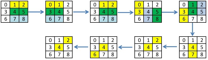
With a little thought, you can improve sorting by doing the same operations only once. For clarity, I will show what sorting was and what became, and what are the benefits of this approach.
In a previous post, I used the already invented incomplete Butcher sorting for 9 elements, which allows you to find the median without using conditional operators for the minimum number of operations. We represent this sorting in the form of iterations, on each of which independent elements are sorted, but there are dependencies between iterations. For each iteration, pairs of elements for sorting are selected.
Old sort:
New Sort:

In appearance, both approaches can be said to be the same. But let's look at this from the point of view of optimization in terms of the number of operations and the ability to use the calculated values by other threads. You can load and sort columns only once, make exchanges between threads and count the median. This will visually look like this:
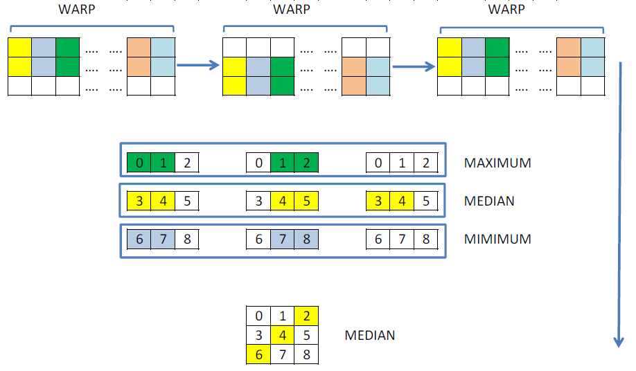
The following kernel corresponds to such an algorithm. For exchanges, I decided to use not shared memory, but new __shfl operations, which allow you to exchange values inside one warp without synchronization. Thus, it is possible to partially avoid doing repeated calculations.
__global__ BOUNDS(BL_X, 2048 / BL_X)
void mFilter_3x3(const int H, const int W, const unsigned char * __restrict in, unsigned char *out)
{
    // индекс по Оси Х
    int idx = threadIdx.x + blockIdx.x * blockDim.x;
    // смещаемся немного назад, так как в каждом warp'е первая и последняя нить не участвует в итоговом вычислении
    idx = idx - 2 * (idx / 32);
    // умножаем на 4, так как мы обрабатываем по 4 точки сразу
    int idy = threadIdx.y + blockIdx.y * blockDim.y * 4 + 1;
    unsigned a[9];
    unsigned RE[3];
    // первая и последняя нить не участвует в итоговом вычислении
    bool bound = (idxW > 0 && idxW < 31 && idx < W - 1);
    // считываем и сортируем столбцы
    RE[0] = in[(idy - 1) * W + idx] | (in[(idy + 0) * W + idx] << 8) | (in[(idy + 1) * W + idx] << 16) | (in[(idy + 2) * W + idx] << 24);
    RE[1] = in[(idy + 0) * W + idx] | (in[(idy + 1) * W + idx] << 8) | (in[(idy + 2) * W + idx] << 16) | (in[(idy + 3) * W + idx] << 24);
    RE[2] = in[(idy + 1) * W + idx] | (in[(idy + 2) * W + idx] << 8) | (in[(idy + 3) * W + idx] << 16) | (in[(idy + 4) * W + idx] << 24);
    Sort(RE[0], RE[1]);
    Sort(RE[1], RE[2]);
    Sort(RE[0], RE[1]);
    // делаем обмены
    a[0] = __shfl_down(RE[0], 1);
    a[1] = RE[0];
    a[2] = __shfl_up(RE[0], 1);
    a[3] = __shfl_down(RE[1], 1);
    a[4] = RE[1];
    a[5] = __shfl_up(RE[1], 1);
    a[6] = __shfl_down(RE[2], 1);
    a[7] = RE[2];
    a[8] = __shfl_up(RE[2], 1);
    // ищем максимум
    a[2] = __vmaxu4(a[0], __vmaxu4(a[1], a[2]));
    // ищем медиану
    Sort(a[3], a[4]);
    a[4] = __vmaxu4(__vminu4(a[4], a[5]), a[3]);
    // ищем минимум
    a[6] = __vminu4(a[6], __vminu4(a[7], a[8]));
    // ищем финально медиану
    Sort(a[2], a[4]);
    a[4] = __vmaxu4(__vminu4(a[4], a[6]), a[2]);
    // записываем результат, если не вышли за границу картинки
    if (idy + 0 < H - 1 && bound)
        out[(idy) * W + idx] = a[4] & 255;
    if (idy + 1 < H - 1 && bound)
        out[(idy + 1) * W + idx] = (a[4] >> 8) & 255;
    if (idy + 2 < H - 1 && bound)
        out[(idy + 2) * W + idx] = (a[4] >> 16) & 255;
    if (idy + 3 < H - 1 && bound)
        out[(idy + 3) * W + idx] = (a[4] >> 24) & 255;
}
The second optimization is related to the fact that each thread can process not 4 points at once, but, for example, 2 sets of 4 points or N sets of 4 points. This is necessary in order to maximize the load of the device, since just for a 3x3 filter, one set of 4 points is not enough.
The third optimization that can still be done is to substitute the width and height of the image. There are several arguments for this:
- Typically, image sizes have fixed values, for example, the popular Full HD, Ultra HD, 720p. You can just have a set of precompiled kernels. This optimization gives about 10-15% to productivity.
- With the Cuda Toolkit 7.5, it’s possible to perform dynamic compilation, which allows you to perform substitution of values at run time.
Fully optimized code will look like this. By varying the number of points, you can get maximum performance. In my case, maximum performance was achieved with numP_char = 3, that is, three sets of 4 points or 12 points per thread.
__global__ BOUNDS(BL_X, 2048 / BL_X)
void mFilter_3x3(const unsigned char * __restrict in, unsigned char *out)
{
    int idx = threadIdx.x + blockIdx.x * blockDim.x;
    idx = idx - 2 * (idx / 32);
    int idxW = threadIdx.x % 32;
    int idy = threadIdx.y + blockIdx.y * blockDim.y * (4 * numP_char) + 1;
    unsigned a[numP_char][9];
    unsigned RE[numP_char][3];
    bool bound = (idxW > 0 && idxW < 31 && idx < W - 1);
#pragma unroll
    for (int z = 0; z < numP_char; ++z)
    {
        RE[z][0] = in[(idy - 1 + z * 4) * W + idx] | (in[(idy - 1 + 1 + z * 4) * W + idx] << 8) | (in[(idy - 1 + 2 + z * 4) * W + idx] << 16) | (in[(idy - 1 + 3 + z * 4) * W + idx] << 24);
        RE[z][1] = in[(idy + z * 4) * W + idx] | (in[(idy + 1 + z * 4) * W + idx] << 8) | (in[(idy + 2 + z * 4) * W + idx] << 16) | (in[(idy + 3 + z * 4) * W + idx] << 24);
        RE[z][2] = in[(idy + 1 + z * 4) * W + idx] | (in[(idy + 1 + 1 + z * 4) * W + idx] << 8) | (in[(idy + 1 + 2 + z * 4) * W + idx] << 16) | (in[(idy + 1 + 3 + z * 4) * W + idx] << 24);
        Sort(RE[z][0], RE[z][1]);
        Sort(RE[z][1], RE[z][2]);
        Sort(RE[z][0], RE[z][1]);
        a[z][0] = __shfl_down(RE[z][0], 1);
        a[z][1] = RE[z][0];
        a[z][2] = __shfl_up(RE[z][0], 1);
        a[z][3] = __shfl_down(RE[z][1], 1);
        a[z][4] = RE[z][1];
        a[z][5] = __shfl_up(RE[z][1], 1);
        a[z][6] = __shfl_down(RE[z][2], 1);
        a[z][7] = RE[z][2];
        a[z][8] = __shfl_up(RE[z][2], 1);
        a[z][2] = __vmaxu4(a[z][0], __vmaxu4(a[z][1], a[z][2]));
        Sort(a[z][3], a[z][4]);
        a[z][4] = __vmaxu4(__vminu4(a[z][4], a[z][5]), a[z][3]);
        a[z][6] = __vminu4(a[z][6], __vminu4(a[z][7], a[z][8]));
        Sort(a[z][2], a[z][4]);
        a[z][4] = __vmaxu4(__vminu4(a[z][4], a[z][6]), a[z][2]);
    }
#pragma unroll
    for (int z = 0; z < numP_char; ++z)
    {
        if (idy + z * 4 < H - 1 && bound)
            out[(idy + z * 4) * W + idx] = a[z][4] & 255;
        if (idy + 1 + z * 4 < H - 1 && bound)
            out[(idy + 1 + z * 4) * W + idx] = (a[z][4] >> 8) & 255;
        if (idy + 2 + z * 4 < H - 1 && bound)
            out[(idy + 2 + z * 4) * W + idx] = (a[z][4] >> 16) & 255;
        if (idy + 3 + z * 4 < H - 1 && bound)
            out[(idy + 3 + z * 4) * W + idx] = (a[z][4] >> 24) & 255;
    }
}
5x5 Median Filter
Unfortunately, I was not able to come up with any other sorting for the 5x5 square. The only thing you can save on is downloading and combining 4 points in an unsigned int. I don’t see the point of bringing an even longer code, since all the transformations can be done by analogy with a 3x3 square.
In this article we describe some of the ideas for the combined operations of the two squares with the imposition of a 20 elements. But the forgetful selection sort method proposed by the authors still does more operations than the incomplete Butcher sorting network for 25 elements, even when combining two adjacent 5x5 squares.
Performance
Finally, I’ll give you some numbers that I was able to get throughout the optimization process.
| Lead time, ms | Acceleration | |||||
|---|---|---|---|---|---|---|
| Scalar CPU | AVX2 CPU | GPU | Scalar / GPU | AVX2 / GPU | ||
| 3x3 1920x1080 | 22.9 | 0.255 | 0.044 (47.1 GP / s) | 520 | 5.8 | |
| 3x3 4096x2160 | 97.9 | 1.33 | 0.172 (51.4 GP / s) | 569 | 7.73 | |
| 5x5 1920x1080 | 134.3 | 1.47 | 0.260 (7.9 GP / s) | 516 | 5.6 | |
| 5x5 4096x2160 | 569.2 | 6.69 | 1.000 (8.8 GP / s) | 569 | 6.69 | |
Conclusion
In conclusion, I want to note that among all the found articles and implementations of median filtering for the GPU, the already mentioned article is of interest"Fine-tuned high-speed implementation of a GPU-based median filter", published in 2013. In this article, the authors proposed a completely different approach to sorting, namely, the forgetful selection method. The essence of this method is that we take roundUp (N / 2) + 1 elements, go from left to right and back, thereby obtaining the minimum and maximum elements at the edges. Next, forget these elements, add one of the remaining elements to the end and repeat the process. When there is already nothing to add, we get an array of 3 elements, from which the median will be easy to select. One of the advantages of this approach is the reduced number of registers used, compared with the known sortings.
The article states that the authors got a result of 1.8 GPixels / sec on the Tesla C2050. The power of this card in single precision is estimated at 1 TFlops. The power of the 780Ti participating in the test is estimated at 5 TFlops. Thus, the specific computational speed per 1 TFlops of the algorithm I proposed is approximately 5.5 times higher for a 3x3 square and 2 times higher for a 5x5 square than that proposed by the authors of the article. This comparison is not entirely correct, but more approximate to the truth. Also in this article it was mentioned that at that time their implementation was the fastest of all known.
The achieved acceleration compared to the AVX2 version averaged 6 times. If you use new cards based on the Pascal architecture, this acceleration can increase at least 2 times, which will be approximately 100 GPixels / sec.