In three articles on the smallest squares: literacy on the theory of probability
- Tutorial
A year and a half ago, I published an article “Mathematics on the fingers: the methods of least squares,” which received a very decent response, which, among other things, consisted in what I suggested to draw an owl. Well, once an owl, then you need to explain again. In a week exactly on this topic I will begin to give several lectures to geological students; I take this opportunity to present here the (adapted) basic theses as a draft. My main goal is not to give a ready-made recipe from a book about tasty and healthy food, but to tell why it is and what else is in the appropriate section, because the connection between different sections of mathematics is the most interesting!
At the moment I intend to break the text into three articles:
I will go to the smallest squares a little to the side, through the maximum likelihood principle, and it requires minimal orientation in probability theory. This text is intended for the third year of our Faculty of Geology, which means (from the point of view of the involved hardware!) That the interested high school student with appropriate diligence should be able to figure it out.
Once I was asked if I believed in the theory of evolution. Pause right now, think about how you answer it.

Personally, I was taken aback, replied that I find it plausible, and that the question of faith does not arise here at all. Scientific theory has little to do with faith. In short, the theory only builds a model of the world around us, there is no need to believe in it. Moreover, the Popper criterionrequires a scientific theory to be able to rebut. And still the well-founded theory should possess, first of all, predictive power. For example, if you genetically modify crops in such a way that they themselves will produce pesticides, then it is logical that insects resistant to them will appear. However, it is significantly less obvious that this process can be slowed down by growing ordinary plants side by side with genetically modified ones. Based on the theory of evolution, the corresponding modeling made such a prediction , and it seems to be confirmed .
As I mentioned earlier, I will go to the smallest squares through the maximum likelihood principle. Let's illustrate with an example. Suppose we are interested in data on the growth of penguins, but we can measure only a few of these beautiful birds. It is quite logical to introduce a growth distribution model into the task - most often it is normal. The normal distribution is characterized by two parameters — the mean value and the standard deviation. For each fixed parameter value, we can calculate the probability that exactly the measurements that we made will be generated. Further, by varying the parameters, we find those that maximize the probability.
Thus, to work with maximum likelihood, we need to operate in terms of probability theory. Below we define the notion of probability and likelihood “on the fingers”, but first I would like to focus on another aspect. I surprisingly rarely see people who think about the word "theory" in the phrase "probability theory."
As to the sources, meanings and range of applicability of probabilistic estimates, fierce disputes have been going on for more than a hundred years. For example, Bruno De Finetti stated that probability is nothing but a subjective analysis of the likelihood that something will happen, and that this probability does not exist outside the mind. This is a person's willingness to bet on something happening. This view is exactly the opposite of the classics / frequentists.on the probability of a specific result of an event in which it is assumed that the same event can be repeated many times, and the “probability” of a particular result is related to the frequency of a particular result during repeated tests. In addition to subjectivists and frequentists, there are also objectivists who assert that probabilities are real aspects of the universe, and not just descriptions of the degree of confidence of the observer.
Be that as it may, but all three scientific schools in practice use the same apparatus, based on Kolmogorov's axioms. Let's give an indirect argument, from a subjectivist point of view, in favor of the theory of probability, built on Kolmogorov's axioms. We will give the axioms themselves a bit later, but first we assume that we have a bookmaker who accepts bets on the next World Cup. Let us have two events: a = the champion will be the team of Uruguay, b = the champion will be the team of Germany. The bookmaker estimates the chances of the Uruguay team to win at 40%, the chances of the German team at 30%. Obviously, both Germany and Uruguay cannot win at the same time, therefore the chance a∧b is zero. Well, at the same time, the bookmaker believes that the probability that either Uruguay will win, or Germany (and not Argentina or Australia) is 80%.

If the bookmaker claims that his degree of confidence in the event a is equal to 0.4, that is, P (a) = 0.4, then the player can choose whether he will bet for or against the statement a , setting amounts that are compatible with the degree of confidence of the bookmaker. This means that the player can bet that the event a will occur by placing four rubles against the six rubles of the bookmaker. Or the player can put six rubles instead of four rubles bookmaker that event and will not happen.
If the bookmaker’s degree of confidence does not accurately reflect the state of the world, then it can be expected that in the long run he will lose money to players whose beliefs are more accurate. Moreover, in this particular example, the player has a strategy in which the bookmaker always loses money. Let's illustrate it:
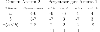
A player makes three bets, and whatever the outcome of the championship, he always wins. Please note that in consideration of the amount of winnings, in principle, it does not include whether Uruguay or Germany are the favorites of the championship, the bookmaker’s loss is guaranteed! This situation was caused by the fact that the bookmaker was not guided by the basics of the theory of probability, violating the third Kolmogorov axiom, let us give them all three:
In text form, they look like this:
In 1931, de Finetti proved a very strong statement:
Probability axioms can be considered as limiting the set of probabilistic beliefs that an agent can hold. Please note that following the bookmaker Kolmogorov's axioms do not imply that he will win (we leave aside commission questions), but if they are not followed, he will be guaranteed to lose. Note that other arguments have been put forward in favor of applying probabilities; but it was precisely the practical success of systems of formation of reasoning based on probability theory that turned out to be an attractive stimulus that caused a revision of many views.
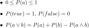
So, we barely opened the veil of whyA teverver may make sense, but what objects exactly does it manipulate? The whole theory is built only on three axioms; in all three, some magic function P is involved . Moreover, looking at these axioms, it reminds me a lot of the function of the area of a figure. Let's try to see if a square works to determine probability.
We define the word "event" as a "subset of unit square." We define the word "probability of an event" as "the area of the corresponding subset." Roughly speaking, we have a large cardboard target, and we close our eyes and shoot at it. The chances of a bullet falling into a given set are directly proportional to the area of the set. A reliable event in this case is the entire square, and a deliberately false, for example, any point of the square. From our definition of probability, it follows that ideally it is impossible to hit a point (our bullet is a material point). I really like pictures, and draw a lot of them, and theorever is no exception! Let's illustrate all three axioms:
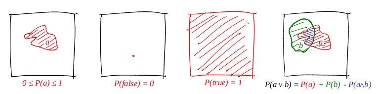
So, the first axiom is fulfilled: the area is non-negative, and cannot exceed unity. A credible event is the whole square, and a deliberately false one is any set of zero area. And it works great with disjunctice!
Let's look at the simplest example of a coin toss, aka Bernoulli scheme . N experiments are conducted , in each of which one of two events can occur (“success” or “failure”), one with probability p , the second with probability 1-p . Our task is to find the probability of obtaining exactly k successes in these n experiments. This probability is given by the Bernoulli formula:

Let's take a regular coin ( p = 0.5 ), throw it ten times ( n = 10 ), and count how many times the tail falls:
This is how the probability density plot looks like:
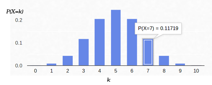
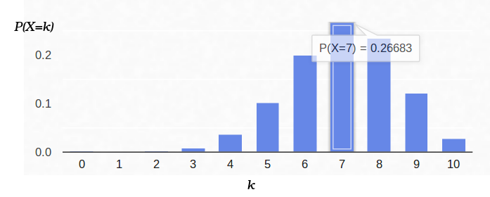
Thus, if we recorded the probability of “success” (0.5), and also recorded the number of experiments (10), then the possible number of “successes” can be any integer between 0 and 10, but these outcomes are not equally probable. It is quite obvious that getting five “successes” is much more likely than none. For example, the probability to count seven tails is approximately 12%.
And now let's look at the same task from the other side. We have a real coin, but we don’t know its distribution of the prior probability of “success” / “failure”. However, we can throw it ten times and count the number of "success." For example, we had seven tails. How does this help us evaluate p ?
We can try to fix in the formula Bernoulli n= 10 and k = 7, leaving p free parameter:

Then the Bernoulli formula can be interpreted as the likelihood of the parameter being evaluated (in this case p ). I even changed the letter from the function, now it is L (from English like like). That is, the likelihood is the probability of generating observation data (7 tails of 10 experiments) for a given value of the parameter (s).
For example, the likelihood of a balanced coin ( p = 0.5) under the condition that seven tails of ten shots fall out is approximately equal to 12%. You can plot the function L :
So, we are looking for such a parameter value that maximizes the likelihood of obtaining those observations that we have. In this particular case, we have a function of one variable, we are looking for its maximum. In order to make it easier to search, I will seek the maximum no of L , and the log of L . The logarithm is a strictly monotonic function, so maximization of the one and the other is strictly the same. And the logarithm of us breaks the product into an amount that is much more convenient to differentiate. So, we are looking for the maximum of this function:

To do this, we equate its derivative to zero:

Derivative log x = 1 / x, we get:

That is, the maximum likelihood (approximately 27%) is reached at the point.

Just in case we calculate the second derivative:
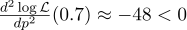
At the point p = 0.7, it is negative, so this point is really the maximum of the function L.
And this is what the probability density looks like for the Bernoulli scheme with p = 0.7:
Let's imagine that we have a certain constant physical quantity that we want to measure, be it with a ruler or voltage with a voltmeter. Any measurement gives an approximation of this value, but not the value itself. The methods that I describe here were developed by Gauss in the late 18th century, when he measured the orbits of celestial bodies.
For example, if we measure the battery voltage N times, we get N different measurements. Which one to take? Everything! So, let us have N values of Uj:

Suppose that each dimension of Uj is equal to the ideal value, plus Gaussian noise, which is characterized by two parameters — the position of the Gaussian bell and its “width”. Here is the probability density:
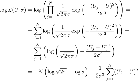
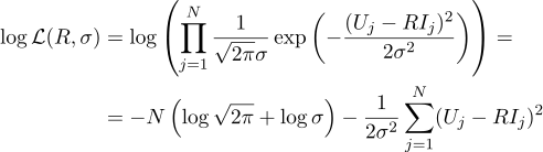
That is, having N given values of Uj, our task is to find such a parameter, U, which maximizes the likelihood value. Likelihood (I immediately take the logarithm from it) can be written as follows:
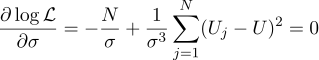
Well, then everything is strictly as before, we equate the partial derivatives with respect to the parameters we are looking for:
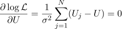
We get that the most likely estimate of the unknown quantity U can be found as the average of all measurements :

Well, the most likely sigma parameter is the usual standard deviation:

Was it worth bothering to get a simple average of all measurements in the answer? For my taste, it was worth it. By the way, averaging multiple measurements of a constant value in order to increase the accuracy of measurements is quite standard practice. For example, ADC averaging. By the way, for this Gaussian noise is not needed, it is enough that the noise is unbiased.
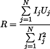
Continuing the conversation, let's take the same example, but slightly complicate it. We want to measure the resistance of a certain resistor. With the help of a laboratory power supply, we are able to pass through it a certain reference amount of amperes, and measure the voltage that will be needed for this. That is, we will have N pairs of numbers (Ij, Uj) at the input of our appraiser.

Draw these points on the graph; Ohm's law tells us that we are looking for the slope of the blue line.
We write the expression for the likelihood of the parameter R:
And again we equate the corresponding partial derivative to zero:
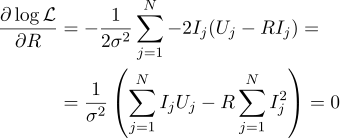
Then the most plausible resistance R can be found by the following formula:
This result is somewhat less obvious than the simple average of all measurements. Please note that if we make a hundred measurements in the region of one amp, and one measurement in the kiloampere region, then the previous hundred measurements will have almost no effect on the result. Let's remember this fact, it will be useful to us in the next article.
Surely you have already noticed that in the last two examples, maximizing the likelihood logarithm is equivalent to minimizing the sum of squares of the estimation error. Let's take another example. Take a calibration balance with reference weights. Suppose we have N reference weights of mass xj, hang them on the barren and measure the length of the spring, we get N spring lengths yj:

Hooke's law tells us that the spring tension linearly depends on the applied force, and this force includes the weight of the goods and weight the spring itself. Let the spring stiffness is the parameter a , well, and the spring tension under its own weight is the parameter b. Then we can write the likelihood expression of our measurements like this (still under the hypothesis of Gaussian measurement noise):
Maximizing the likelihood L is equivalent to minimizing the sum of the squares of estimation errors, that is, we can search for the minimum of the function S defined as follows:
In other words, we are looking for a line that minimizes the sum of the squares of the lengths of the green segments:
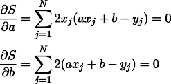
Well, after that, the derivatives:
We obtain a system of two linear equations with two unknowns: We
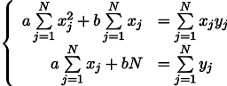
recall the seventh grade of the school and write out the solution:

The least squares methods are a particular case of maximizing the likelihood for those cases where the probability density is Gaussian. In the case when the density is (not at all) Gaussian, the OLS give an estimate that differs from the MLE (maximum likehood estimation) estimate. By the way, at one time Gauss hypothesized that the distribution does not play a role, only the independence of the tests is important.
As can be seen from this article, the further into the forest, the more cumbersome are the analytical solutions to this problem. Well, we are not in the eighteenth century, we have computers! Next time we will see a geometric and, then, a programmer approach to the OLS problem, stay on the line.
At the moment I intend to break the text into three articles:
- 1. Educational program on the theory of probability and how it is connected with the methods of least squares
- 2. The smallest squares, the simplest case, and how to program them
- 3. Nonlinear problems
I will go to the smallest squares a little to the side, through the maximum likelihood principle, and it requires minimal orientation in probability theory. This text is intended for the third year of our Faculty of Geology, which means (from the point of view of the involved hardware!) That the interested high school student with appropriate diligence should be able to figure it out.
How justified is the theorever or do you believe in the theory of evolution?
Once I was asked if I believed in the theory of evolution. Pause right now, think about how you answer it.
Personally, I was taken aback, replied that I find it plausible, and that the question of faith does not arise here at all. Scientific theory has little to do with faith. In short, the theory only builds a model of the world around us, there is no need to believe in it. Moreover, the Popper criterionrequires a scientific theory to be able to rebut. And still the well-founded theory should possess, first of all, predictive power. For example, if you genetically modify crops in such a way that they themselves will produce pesticides, then it is logical that insects resistant to them will appear. However, it is significantly less obvious that this process can be slowed down by growing ordinary plants side by side with genetically modified ones. Based on the theory of evolution, the corresponding modeling made such a prediction , and it seems to be confirmed .
And what have the smallest squares?
As I mentioned earlier, I will go to the smallest squares through the maximum likelihood principle. Let's illustrate with an example. Suppose we are interested in data on the growth of penguins, but we can measure only a few of these beautiful birds. It is quite logical to introduce a growth distribution model into the task - most often it is normal. The normal distribution is characterized by two parameters — the mean value and the standard deviation. For each fixed parameter value, we can calculate the probability that exactly the measurements that we made will be generated. Further, by varying the parameters, we find those that maximize the probability.
Thus, to work with maximum likelihood, we need to operate in terms of probability theory. Below we define the notion of probability and likelihood “on the fingers”, but first I would like to focus on another aspect. I surprisingly rarely see people who think about the word "theory" in the phrase "probability theory."
What is studying teverver?
As to the sources, meanings and range of applicability of probabilistic estimates, fierce disputes have been going on for more than a hundred years. For example, Bruno De Finetti stated that probability is nothing but a subjective analysis of the likelihood that something will happen, and that this probability does not exist outside the mind. This is a person's willingness to bet on something happening. This view is exactly the opposite of the classics / frequentists.on the probability of a specific result of an event in which it is assumed that the same event can be repeated many times, and the “probability” of a particular result is related to the frequency of a particular result during repeated tests. In addition to subjectivists and frequentists, there are also objectivists who assert that probabilities are real aspects of the universe, and not just descriptions of the degree of confidence of the observer.
Be that as it may, but all three scientific schools in practice use the same apparatus, based on Kolmogorov's axioms. Let's give an indirect argument, from a subjectivist point of view, in favor of the theory of probability, built on Kolmogorov's axioms. We will give the axioms themselves a bit later, but first we assume that we have a bookmaker who accepts bets on the next World Cup. Let us have two events: a = the champion will be the team of Uruguay, b = the champion will be the team of Germany. The bookmaker estimates the chances of the Uruguay team to win at 40%, the chances of the German team at 30%. Obviously, both Germany and Uruguay cannot win at the same time, therefore the chance a∧b is zero. Well, at the same time, the bookmaker believes that the probability that either Uruguay will win, or Germany (and not Argentina or Australia) is 80%.
If the bookmaker claims that his degree of confidence in the event a is equal to 0.4, that is, P (a) = 0.4, then the player can choose whether he will bet for or against the statement a , setting amounts that are compatible with the degree of confidence of the bookmaker. This means that the player can bet that the event a will occur by placing four rubles against the six rubles of the bookmaker. Or the player can put six rubles instead of four rubles bookmaker that event and will not happen.
If the bookmaker’s degree of confidence does not accurately reflect the state of the world, then it can be expected that in the long run he will lose money to players whose beliefs are more accurate. Moreover, in this particular example, the player has a strategy in which the bookmaker always loses money. Let's illustrate it:
A player makes three bets, and whatever the outcome of the championship, he always wins. Please note that in consideration of the amount of winnings, in principle, it does not include whether Uruguay or Germany are the favorites of the championship, the bookmaker’s loss is guaranteed! This situation was caused by the fact that the bookmaker was not guided by the basics of the theory of probability, violating the third Kolmogorov axiom, let us give them all three:
In text form, they look like this:
- 1. All probabilities range from 0 to 1
- 2. Certainly true statements have probability 1, and certainly false probability 0.
- 3. The third axiom is an axiom of disjunction, it is easy to intuitively understand it, noting that those cases when the statement a is true, together with those cases when b is true, unconditionally covers all those cases when the true statement a∨b; but in the sum of two sets of cases, their intersection occurs twice, so it is necessary to subtract P (ab).
In 1931, de Finetti proved a very strong statement:
If a bookmaker is guided by a set of degrees of confidence that violates the axioms of probability theory, then there is such a combination of player bets that guarantees the loss of a bookmaker (player's win) at each bet.
Probability axioms can be considered as limiting the set of probabilistic beliefs that an agent can hold. Please note that following the bookmaker Kolmogorov's axioms do not imply that he will win (we leave aside commission questions), but if they are not followed, he will be guaranteed to lose. Note that other arguments have been put forward in favor of applying probabilities; but it was precisely the practical success of systems of formation of reasoning based on probability theory that turned out to be an attractive stimulus that caused a revision of many views.
So, we barely opened the veil of whyA teverver may make sense, but what objects exactly does it manipulate? The whole theory is built only on three axioms; in all three, some magic function P is involved . Moreover, looking at these axioms, it reminds me a lot of the function of the area of a figure. Let's try to see if a square works to determine probability.
We define the word "event" as a "subset of unit square." We define the word "probability of an event" as "the area of the corresponding subset." Roughly speaking, we have a large cardboard target, and we close our eyes and shoot at it. The chances of a bullet falling into a given set are directly proportional to the area of the set. A reliable event in this case is the entire square, and a deliberately false, for example, any point of the square. From our definition of probability, it follows that ideally it is impossible to hit a point (our bullet is a material point). I really like pictures, and draw a lot of them, and theorever is no exception! Let's illustrate all three axioms:
So, the first axiom is fulfilled: the area is non-negative, and cannot exceed unity. A credible event is the whole square, and a deliberately false one is any set of zero area. And it works great with disjunctice!
Maximum likelihood by example
Example one: coin flip
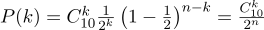
Let's look at the simplest example of a coin toss, aka Bernoulli scheme . N experiments are conducted , in each of which one of two events can occur (“success” or “failure”), one with probability p , the second with probability 1-p . Our task is to find the probability of obtaining exactly k successes in these n experiments. This probability is given by the Bernoulli formula:
Let's take a regular coin ( p = 0.5 ), throw it ten times ( n = 10 ), and count how many times the tail falls:
This is how the probability density plot looks like:
Thus, if we recorded the probability of “success” (0.5), and also recorded the number of experiments (10), then the possible number of “successes” can be any integer between 0 and 10, but these outcomes are not equally probable. It is quite obvious that getting five “successes” is much more likely than none. For example, the probability to count seven tails is approximately 12%.
And now let's look at the same task from the other side. We have a real coin, but we don’t know its distribution of the prior probability of “success” / “failure”. However, we can throw it ten times and count the number of "success." For example, we had seven tails. How does this help us evaluate p ?
We can try to fix in the formula Bernoulli n= 10 and k = 7, leaving p free parameter:
Then the Bernoulli formula can be interpreted as the likelihood of the parameter being evaluated (in this case p ). I even changed the letter from the function, now it is L (from English like like). That is, the likelihood is the probability of generating observation data (7 tails of 10 experiments) for a given value of the parameter (s).
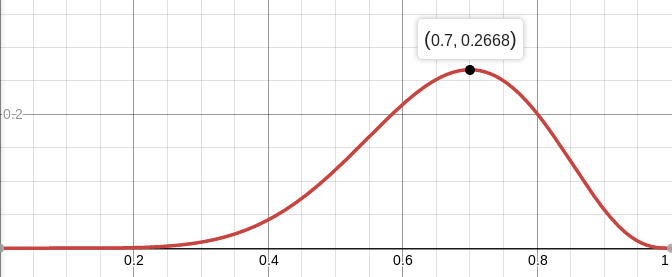
For example, the likelihood of a balanced coin ( p = 0.5) under the condition that seven tails of ten shots fall out is approximately equal to 12%. You can plot the function L :
So, we are looking for such a parameter value that maximizes the likelihood of obtaining those observations that we have. In this particular case, we have a function of one variable, we are looking for its maximum. In order to make it easier to search, I will seek the maximum no of L , and the log of L . The logarithm is a strictly monotonic function, so maximization of the one and the other is strictly the same. And the logarithm of us breaks the product into an amount that is much more convenient to differentiate. So, we are looking for the maximum of this function:
To do this, we equate its derivative to zero:
Derivative log x = 1 / x, we get:
That is, the maximum likelihood (approximately 27%) is reached at the point.
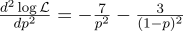
Just in case we calculate the second derivative:
At the point p = 0.7, it is negative, so this point is really the maximum of the function L.
And this is what the probability density looks like for the Bernoulli scheme with p = 0.7:
Example Two: ADC
Let's imagine that we have a certain constant physical quantity that we want to measure, be it with a ruler or voltage with a voltmeter. Any measurement gives an approximation of this value, but not the value itself. The methods that I describe here were developed by Gauss in the late 18th century, when he measured the orbits of celestial bodies.
For example, if we measure the battery voltage N times, we get N different measurements. Which one to take? Everything! So, let us have N values of Uj:
Suppose that each dimension of Uj is equal to the ideal value, plus Gaussian noise, which is characterized by two parameters — the position of the Gaussian bell and its “width”. Here is the probability density:
That is, having N given values of Uj, our task is to find such a parameter, U, which maximizes the likelihood value. Likelihood (I immediately take the logarithm from it) can be written as follows:
Well, then everything is strictly as before, we equate the partial derivatives with respect to the parameters we are looking for:
We get that the most likely estimate of the unknown quantity U can be found as the average of all measurements :
Well, the most likely sigma parameter is the usual standard deviation:
Was it worth bothering to get a simple average of all measurements in the answer? For my taste, it was worth it. By the way, averaging multiple measurements of a constant value in order to increase the accuracy of measurements is quite standard practice. For example, ADC averaging. By the way, for this Gaussian noise is not needed, it is enough that the noise is unbiased.
Example three, and again one-dimensional
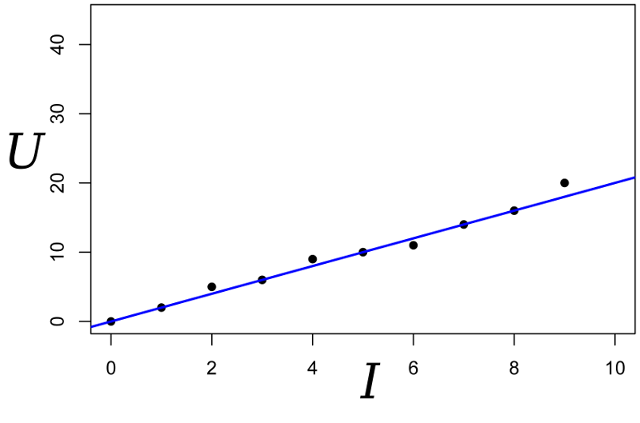
Continuing the conversation, let's take the same example, but slightly complicate it. We want to measure the resistance of a certain resistor. With the help of a laboratory power supply, we are able to pass through it a certain reference amount of amperes, and measure the voltage that will be needed for this. That is, we will have N pairs of numbers (Ij, Uj) at the input of our appraiser.
Draw these points on the graph; Ohm's law tells us that we are looking for the slope of the blue line.
We write the expression for the likelihood of the parameter R:
And again we equate the corresponding partial derivative to zero:
Then the most plausible resistance R can be found by the following formula:
This result is somewhat less obvious than the simple average of all measurements. Please note that if we make a hundred measurements in the region of one amp, and one measurement in the kiloampere region, then the previous hundred measurements will have almost no effect on the result. Let's remember this fact, it will be useful to us in the next article.
Fourth example: back to the smallest squares
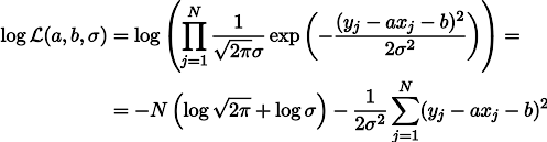
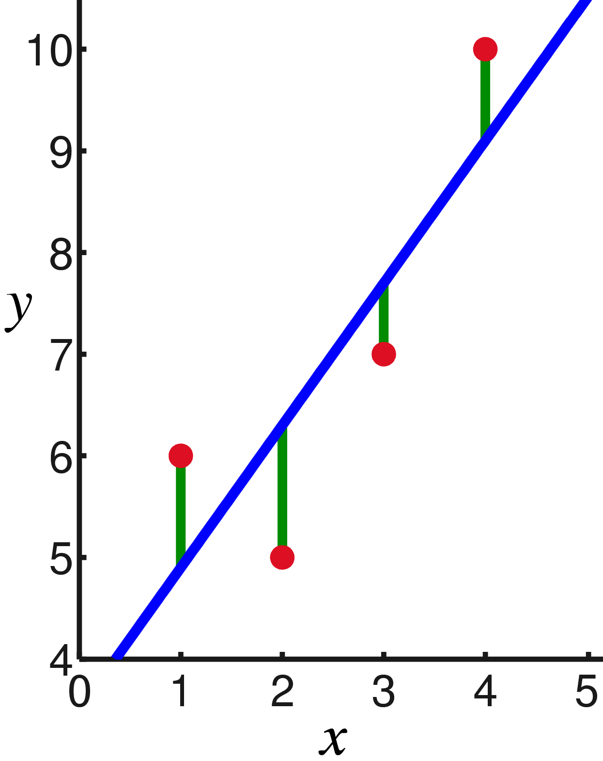
Surely you have already noticed that in the last two examples, maximizing the likelihood logarithm is equivalent to minimizing the sum of squares of the estimation error. Let's take another example. Take a calibration balance with reference weights. Suppose we have N reference weights of mass xj, hang them on the barren and measure the length of the spring, we get N spring lengths yj:
Hooke's law tells us that the spring tension linearly depends on the applied force, and this force includes the weight of the goods and weight the spring itself. Let the spring stiffness is the parameter a , well, and the spring tension under its own weight is the parameter b. Then we can write the likelihood expression of our measurements like this (still under the hypothesis of Gaussian measurement noise):
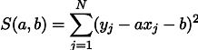
Maximizing the likelihood L is equivalent to minimizing the sum of the squares of estimation errors, that is, we can search for the minimum of the function S defined as follows:
In other words, we are looking for a line that minimizes the sum of the squares of the lengths of the green segments:
Well, after that, the derivatives:
We obtain a system of two linear equations with two unknowns: We
recall the seventh grade of the school and write out the solution:
Conclusion
The least squares methods are a particular case of maximizing the likelihood for those cases where the probability density is Gaussian. In the case when the density is (not at all) Gaussian, the OLS give an estimate that differs from the MLE (maximum likehood estimation) estimate. By the way, at one time Gauss hypothesized that the distribution does not play a role, only the independence of the tests is important.
As can be seen from this article, the further into the forest, the more cumbersome are the analytical solutions to this problem. Well, we are not in the eighteenth century, we have computers! Next time we will see a geometric and, then, a programmer approach to the OLS problem, stay on the line.