Machine Learning Algorithm Brief Review of the Support Vectors Vectors (SVM)
- Tutorial
Foreword

In this article, we will explore several aspects of SVM:
- theoretical component of SVM;
- how the algorithm works on samples that cannot be broken down into class or linear;
- An example of using in Python and the implementation of the algorithm in the library SciKit Learn.
In the following articles, I will try to talk about the mathematical component of this algorithm.
As you know, machine learning tasks are divided into two main categories - classification and regression. Depending on which of these tasks we are facing, and which one we have in our data for this task, we choose which algorithm to use.
The Support Vector Vectors or SVM method (from the English. Support Vector Machines) is a linear algorithm used in classification and regression problems. This algorithm has wide application in practice and can solve both linear and nonlinear problems. The essence of the work of the “Machines” Support Vectors is simple: the algorithm creates a line or hyperplane that divides the data into classes.
Theory
The main task of the algorithm is to find the most correct line, or hyperplane, which divides the data into two classes. An SVM is an algorithm that receives input data and returns such a dividing line.
Consider the following example. Suppose we have a data set, and we want to classify and divide the red squares from the blue circles (for example, positive and negative). The main goal in this task will be to find the “ideal” line that will separate these two classes.
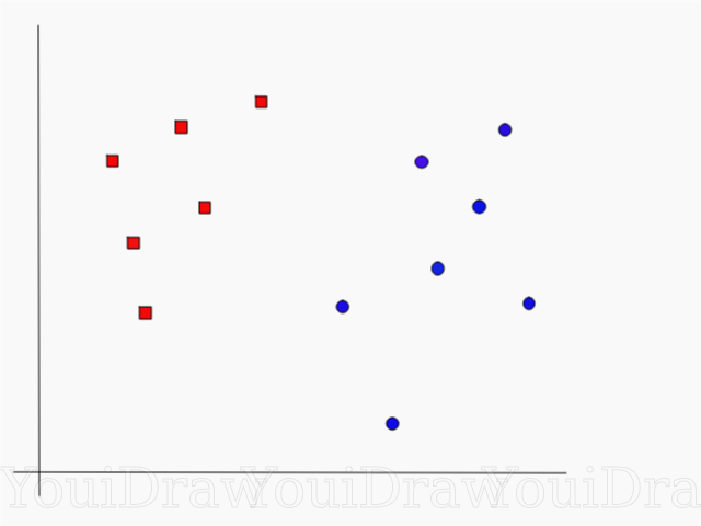
Find the perfect line, or hyperplane, that divides the data set into blue and red classes.
At first glance, it's not so difficult, right?
But, as you can see, there is no one, unique line that would solve such a problem. We can pick up an infinite number of such lines that can divide these two classes. How exactly does SVM find the “ideal” line, and what does the “ideal” mean in its understanding?
Take a look at the example below, and think which of the two lines (yellow or green) best separates the two classes, and fits the description of the “ideal”?
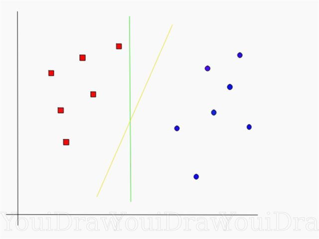
Which line best separates the data set in your opinion?
If you choose the yellow straight, I congratulate you: this is the very line that the algorithm would choose. In this example, we can intuitively understand that the yellow line separates and accordingly classifies the two classes better than the green.
In the case of the green line - it is too close to the red class. Despite the fact that it correctly classified all the objects of the current data set, such a line will not be generalized - it will not behave as well with an unfamiliar data set. The task of finding a generalized separating two classes is one of the main tasks in machine learning.
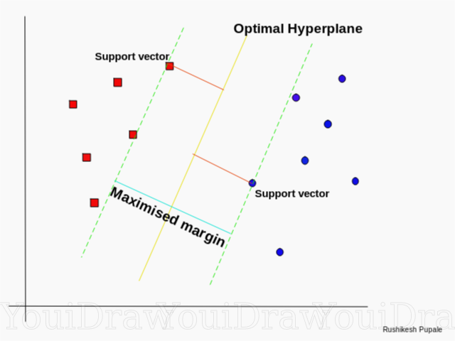
How SVM finds the best line
The SVM algorithm is designed in such a way that it looks for points on the graph that are located directly to the dividing line closest. These points are called support vectors. Then, the algorithm calculates the distance between the reference vectors and the dividing plane. This distance is called the gap. The main goal of the algorithm is to maximize the clearance distance. The best hyperplane is such a hyperplane, for which this gap is as large as possible.
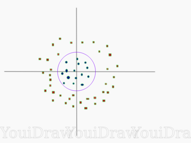
Pretty simple, isn't it? Consider the following example, with a more complex dataset that cannot be divided linearly.
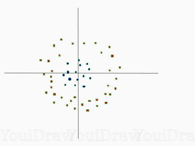
Obviously, this data set cannot be divided linearly. We cannot draw a straight line that would classify this data. But, this dataset can be divided linearly by adding an additional dimension, which we will call the Z axis. Imagine that the coordinates on the Z axis are governed by the following constraint:
Thus, the ordinate Z is represented from the square of the distance of the point to the beginning of the axis.
Below is a visualization of the same data set, on the Z axis.
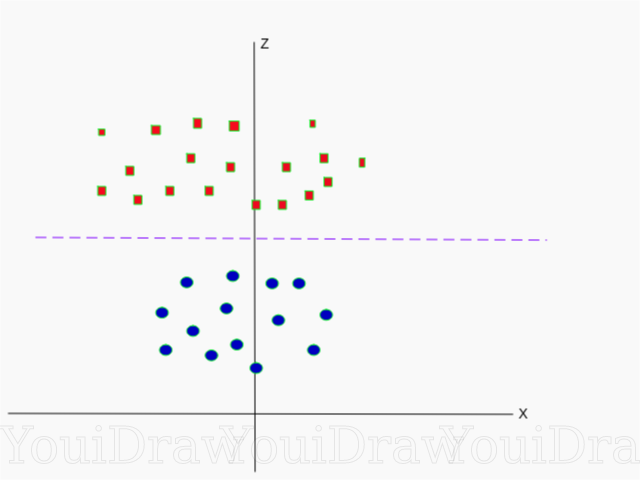
Now the data can be divided linearly. Suppose the magenta line separates the data z = k, where k is a constant. If athen - the formula of a circle. In this way, we can design our linear separator, back to the original number of sample dimensions, using this transformation.
As a result, we can classify a non-linear data set by adding an additional dimension to it, and then, bring it back to its original form using a mathematical transformation. However, not with all data sets it is possible to rotate such a transformation with the same ease. Fortunately, the implementation of this algorithm in the sklearn library solves this problem for us.
Hyperplane
Now that we are familiar with the logic of the algorithm, let's move on to the formal definition of a hyperplane.
A hyperplane is an n-1 dimensional subplane in an n-dimensional Euclidean space that divides space into two separate parts.
For example, imagine that our line is represented as a one-dimensional Euclidean space (i.e., our data set lies on a straight line). Select a point on this line. This point will divide the data set, in our case the line, into two parts. The line has one measure, and the point has 0 measures. Therefore, the point is the hyperplane of the line.
For the two-dimensional dataset we met earlier, the dividing line was the same hyperplane. Simply put, for an n-dimensional space, there is an n-1 dimensional hyperplane that divides this space into two parts.
CODE
import numpy as np
X = np.array([[-1, -1], [-2, -1], [1, 1], [2, 1]])
y = np.array([1, 1, 2, 2])
The points are represented as an array of X, and the classes to which they belong as an array of y.
Now we will train our model with this sample. For this example, I set the linear parameter of the “kernel” of the classifier (kernel).
from sklearn.svm import SVC
clf = SVC(kernel='linear')
clf = SVC.fit(X, y)
Predicting the class of a new object
prediction = clf.predict([[0,6]])Settings
Parameters are the arguments you pass when creating a classifier. Below, I have listed some of the most important SVM tunable parameters:
“C”
This parameter helps to adjust that fine line between “smoothness” and the accuracy of the classification of objects in the training set. The higher the value of “C”, the more objects of the training set will be correctly classified.
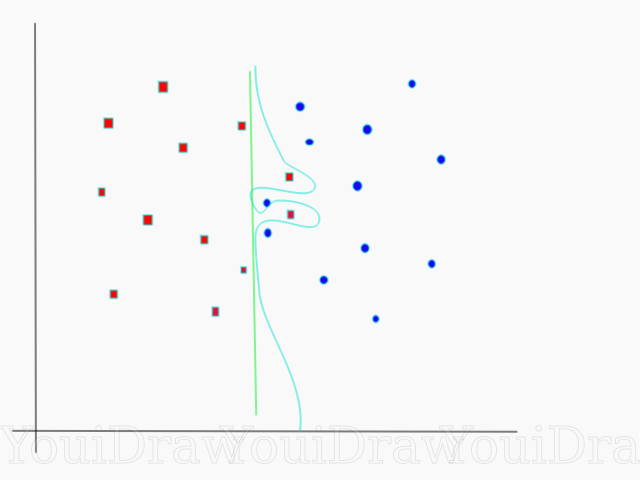
In this example, there are several decision thresholds that we can determine for this particular sample. Pay attention to the straight (represented on the graph as a green line) decision threshold. It is pretty simple, and for this reason, several objects were classified incorrectly. These points that were classified incorrectly are called outliers in the data.
We can also adjust the parameters in such a way that eventually we will get a more curved line (light blue decision threshold) that will classify all the training sample data correctly. Of course, in this case, the chances that our model will be able to generalize and show equally good results on new data are catastrophically small. Therefore, if you are trying to achieve accuracy when training a model, you should aim at something more even, direct. The higher the number “C”, the more entangled the hyperplane will be in your model, but the higher the number of correctly-classified objects of the training set. Therefore, it is important to “tweak” the model parameters for a specific data set in order to avoid retraining but at the same time achieve high accuracy.
Gamma
In the official documentation, the SciKit Learn library states that gamma determines how far each of the elements in a data set has an impact in defining the “perfect line”. The lower the gamma, the more elements, even those that are quite far from the dividing line, take part in the process of choosing this very line. If the gamma is high, then the algorithm will “rely” only on those elements that are closest to the line itself.
If you set the gamma level to be too high, then only the elements closest to the line will participate in the process of deciding on the location of the line. This will help to ignore outliers in the data. The SVM algorithm is designed in such a way that the points located most closely relative to each other have more weight when making decisions. However, with the correct setting of “C” and “gamma”, it is possible to achieve an optimal result, which will build a more linear hyperplane ignoring outliers, and therefore more generalizable.
Conclusion
I sincerely hope that this article helped you to understand the essence of the work of SVM or the Support Vector Vectors Method. I expect any comments and advice from you. In subsequent publications, I will talk about the mathematical component of SVM and optimization problems.
Sources:
Official SVM Documentation in SciKit Learn Siraj Raval
TowardsDataScience Blog
: Support Vector Machines
Intro to Machine Learning Udacity Course Video on SVM: Gamma
Wikipedia: SVM