How to clean up a mailbox using a neural network. Part 2

In our blog, we write a lot about creating email newsletters and working with email. In the modern world, people receive a lot of letters, and in full growth there is a problem with their classification and organization of the mailbox. A US engineer Andrei Kurenkov in his blog talked about how he solved this problem using a neural network. We decided to highlight the progress of this project - a few days ago we published the first part of the story , and today we present to you its continuation.
Deep learning is not suitable here
When Kurenkov first began to study the Keras code, he thought (erroneously) that he would use a sequence reflecting the actual word order in the texts. It turned out that this is not so, but this does not mean that such an option is impossible. What is really worth noting in the field of machine learning is recurrent neural networks that are great for working with large sequences of data, the author writes. This approach implies that when working with words, a “preparatory” step is performed, at which each word is converted into a numerical vector so that similar words go into similar vectors.
Due to this, instead of converting letters to matrices of binary signs, you can simply replace words with numbers using the frequencies of their appearance in letters, and the numbers themselves with vectors that reflect the “meaning” of each word. Then it becomes possible to use the resulting sequence to train a recurrent neural network such as Long Short Term Memory or Gated Recurrent. And this approach has already been implemented : you can simply run the sample and see what happens:
Epoch 1/15
7264/7264 [===========================] - 1330s - loss: 2.3454 - acc: 0.2411 - val_loss: 2.0348 - val_acc: 0.3594
Epoch 2/15
7264/7264 [===========================] - 1333s - loss: 1.9242 - acc: 0.4062 - val_loss: 1.5605 - val_acc: 0.5502
Epoch 3/15
7264/7264 [===========================] - 1337s - loss: 1.3903 - acc: 0.6039 - val_loss: 1.1995 - val_acc: 0.6568
...
Epoch 14/15
7264/7264 [===========================] - 1350s - loss: 0.3547 - acc: 0.9031 - val_loss: 0.8497 - val_acc: 0.7980
Epoch 15/15
7264/7264 [===========================] - 1352s - loss: 0.3190 - acc: 0.9126 - val_loss: 0.8617 - val_acc: 0.7869
Test score: 0.861739277323
Accuracy: 0.786864931846
Training took an eternity, while the result was far from so good. Presumably, the reason may be that there was little data, and the sequences as a whole were not effective enough to categorize them. This means that the increased complexity of learning on sequences does not pay off by the advantage of processing the words of the text in the correct order (nevertheless, the sender and certain words in the letter show well which category it belongs to).
But the additional “preparatory” step still seemed useful to the engineer, since it created a wider representation of the word. Therefore, he considered it worth trying to use it, connecting a convolution to search for important local signs. And again an example was foundKeras, which performs the preparatory step and at the same time transfers the obtained vectors to the convolution and subsampling layers instead of the LSTM layers. But the results are again not impressive:
Epoch 1/3
5849/5849 [===========================] - 127s - loss: 1.3299 - acc: 0.5403 - val_loss: 0.8268 - val_acc: 0.7492
Epoch 2/3
5849/5849 [===========================] - 127s - loss: 0.4977 - acc: 0.8470 - val_loss: 0.6076 - val_acc: 0.8415
Epoch 3/3
5849/5849 [===========================] - 127s - loss: 0.1520 - acc: 0.9571 - val_loss: 0.6473 - val_acc: 0.8554
Test score: 0.556200767488
Accuracy: 0.858725761773 The
engineer really hoped that training using sequences and preparatory steps would prove better than the N-gram model, since theoretically sequences contain more information about the letters themselves. But the widespread belief that deep learning is not very effective for small data sets turned out to be fair.
All because of the signs, fool
So, the tests carried out did not give the desired accuracy of 90% ... As you can see, the current approach to determining attributes from 2500 of the most common words is not suitable, since it includes such general words as “I” or “what” along with useful category-specific words type of "homework". But it’s risky just to remove popular words or reject some sets of words - you never know what will be useful for identifying signs, because, perhaps, sometimes I use this or that “simple” word in one of the categories more often than in others (for example , in the "Personal" section).
Here you need to move from fortune-telling to using the feature selection method to select words that are really good, and filter out words that don't work. The easiest way to do this is to use scikit and its SelectKBest class .which is so fast that the selection takes a minimum of time compared to the operation of a neural network. So will this help?
Dependence of test accuracy on the number of words processed:
Works - 90%!
Excellent! Despite the small differences in the overall performance, it is clearly better to start with a larger set of words. However, this set can be quite significantly reduced by selecting features and not lose performance. Apparently, this neural network has no problems with retraining. Examination of the “best and worst” words according to the version of the program confirms that it defines them well enough:
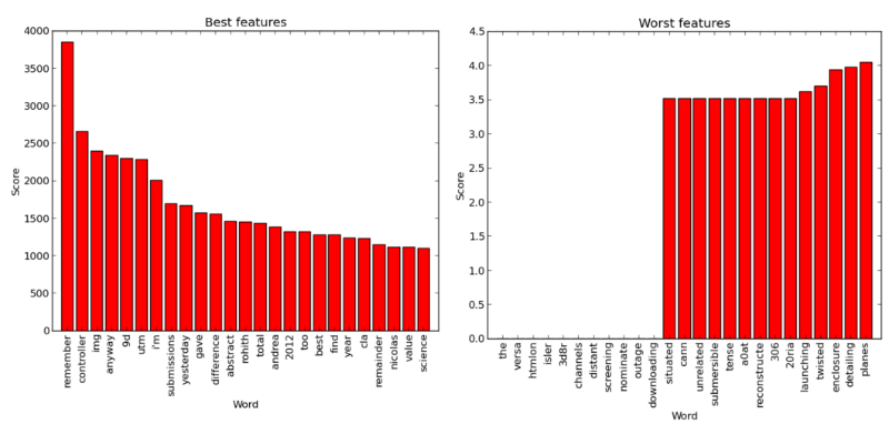
“Best” and “worst” words: selection of signs using the chi-square criterion (based on the code from the scikit example )
Many “good” words, as one would expect, are names or specific terms (for example, “controller”), although Kurenkov says that he would not choose some words like “remember” or “total”. The “worst” words, on the other hand, are fairly predictable, as they are either too general or too rare.
To summarize: the more words, the better, and selecting features can help make the job faster. It helps, but maybe there is a way to further increase the test results. To find out, the engineer decided to take a look at what errors does the neural network, the error matrix, also taken from scikit learn :
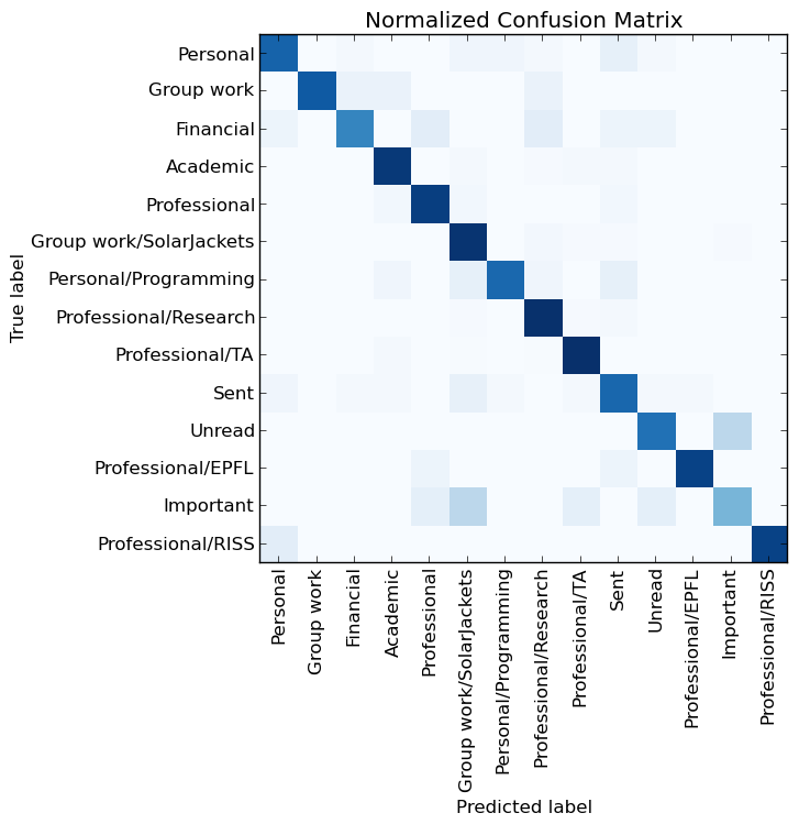
error matrix for the results of the neural network
Great, most color blocks are located diagonally, but there are a few other “annoying spots.” In particular, on visualization the categories “Unread” and “Important” are marked as problematic. But wait! I did not create these categories, and I do not care how well the system handles both them and the Sent category. Undoubtedly, I have to remove them and see how well the neural network works precisely with the categories I created.
Therefore, let's conduct the last experiment in which all the inappropriate categories are absent, and where the largest number of attributes will be used - 10,000 words with a selection of 4,000 of the best:
Epoch 1/5
5850/5850 [===============================] - 2s - loss: 0.8013 - acc: 0.7879 - val_loss: 0.2976 - val_acc: 0.9369
Epoch 2/5
5850/5850 [==============================] - 1s - loss: 0.1953 - acc: 0.9557 - val_loss: 0.2322 - val_acc: 0.9508
Epoch 3/5
5850/5850 [==============================] - 1s - loss: 0.0988 - acc: 0.9795 - val_loss: 0.2418 - val_acc: 0.9338
Epoch 4/5
5850/5850 [==============================] - 1s - loss: 0.0609 - acc: 0.9865 - val_loss: 0.2275 - val_acc: 0.9462
Epoch 5/5
5850/5850 [===============================] - 1s - loss: 0.0406 - acc: 0.9925 - val_loss: 0.2326 - val_acc: 0.9462
722/722 [===============================] - 0s
Test score: 0.243211859068
Accuracy: 0.940443213296 Error
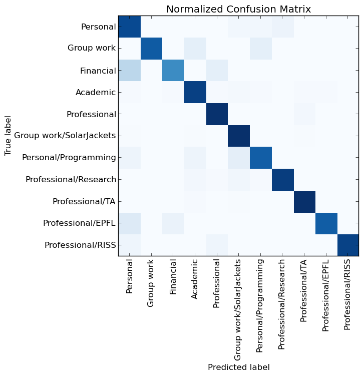
matrix for new neural network results
That's it! A neural network can guess categories with 94% accuracy. Although the effect is primarily due to a large set of attributes, a good classifier (the scikit learn Passive Agressive classifier ) in itself gives 91% accuracy on the same input data. In fact, there are ideas that, in this case, may be effective, and a support vector machine (LinearSVC), - using it, can also be about 94% accuracy.
So, the conclusion is quite simple - “trendy” machine learning methods are not particularly effective on small data sets, and old approaches like N-gram + TF-IFD + SVM can work just as well as modern neural networks. In short, just using the Bag of Words method will work quite well, provided that there are few letters and they are sorted as clearly as in the example above.
Perhaps few people use categories in gmail, but if creating a good classifier is really that simple, it would be nice if gmail had a machine-learning system that defines the category of each letter for organizing mail in one click. At this stage, Kurenkov was very pleased that he had improved his own results by 20% and met Keras in the process.
Epilogue: Additional experiments
While working on his experiment, the engineer did something else. He ran into a problem: all the calculations were carried out for a long time, for the most part because the author of the material did not use the now ordinary trick to start machine learning using the GPU. Following excellent guidance , he did this and got excellent results:
Time spent on achieving the above 90% with and without a GPU; great acceleration!
It should be noted that the Keras neural network, demonstrating 94% accuracy, was much faster to train (and work with) than the network learning on the basis of the support vector method; the first turned out to be the best solution of all that I tried.
The engineer wanted to visualize something else besides the error matrix. In this regard, little has been achieved with Keras, although the author also came across a discussion of visualization issues . This led me to a fork of Keras with a good option for displaying the learning process. He is not very effective, but curious. After a small change in it, he generated excellent training schedules: The
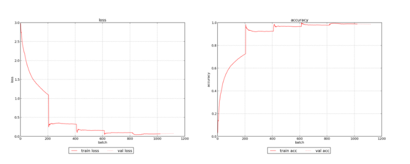
progress of training a neural network using a slightly modified example (with a large number of processed words)
Here you can clearly see how the accuracy of training tends to unity and aligns.
Not bad, but the engineer was more concerned about the increase in accuracy. As before, the first thing he asked was: “Is it possible to quickly change the presentation of features to help the neural network?” The Keras module, which converts text into matrices, has several options in addition to creating binary matrices: matrices with word counts, frequencies or TF-IDF values.
Changing the number of words stored in matrices in the form of signs was also not difficult, so Kurenkov wrote several cycles evaluating how the type of signs and the number of words affect the accuracy of tests. It turned out an interesting graph: The
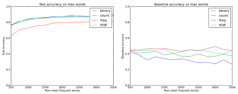
accuracy of the test depending on the type of features and how many words are taken as features (the basic accuracy takes into account k nearest "neighbors")
Here for the first time it became clear that it was necessary to increase the number of words to a value in excess of 1,000. It was also interesting to see that the type of features, characterized by simplicity and the lowest information density (binary), turned out to be no worse and even better than other types that transmit more information about the data .
Although this is fairly predictable - most likely, more interesting words such as “code” or “grade” are useful for categorizing letters, and a single occurrence in the letter is as important as a larger number of references. Without a doubt, the presence of informative features may be useful, but it may also lower the test results due to the increased likelihood of retraining.
In general, we see that binary signs have shown themselves better than others and that increasing the number of words perfectly helps achieve 87% -88% accuracy.
The engineer also looked at the basic algorithms to make sure that something like the k-nearest-neighbor method ( scikit ) is not (in terms of efficiency) the equivalent of neural networks - this turned out to be true. Linear regression worked even worse, so the choice of neural networks is well founded.
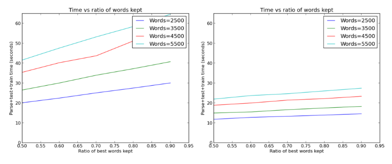
The increase in the number of words, by the way, is not in vain. Even with a cached version of the data, when it was not necessary to parse mail and retrieve attributes each time, the launch of all these tests took a lot of time:
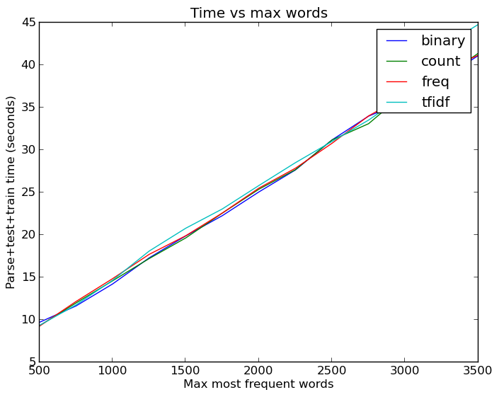
A linear dependence of time growth on the number of words. Actually not bad, with linear regression it was much worse
The increase in the number of words helped, but the experimenter still could not reach the desired threshold of 90%. Therefore, the next thought was to stick to 2,500 words and try to change the size of the neural network. In addition, as it turned out, the model from the Keras example has a 50% dropout regularization on the hidden layer: the engineer was interested to see if this really increases the network efficiency. He launched another set of cycles and got another beautiful graph: A
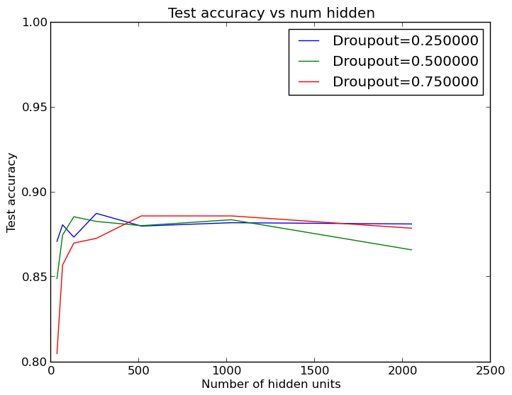
graph of the accuracy change for various options for dropout regularization and hidden layer sizes
It turns out that the size of the hidden layer does not have to be large enough for everything to work as it should! 64 or 124 neurons in the hidden layer can perform the task as well as the standard 512. These results, by the way, are averaged over five starts, so a small spread in the output is not related to the capabilities of small hidden layers.
It follows that a large number of words are needed only to identify useful signs, but there are not so many useful signs themselves - otherwise, for a better result, more neurons would be required. This is good, since we can save a lot of time using smaller hidden layers:

Again, the computation time grows linearly with increasing neurons of the hidden layer
But this is not entirely accurate. Having greater starts with a large number of features engineer discovered that the standard size of the hidden layer (512 neurons) works much better than smaller hidden layers:
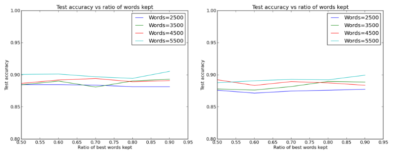
Comparison of the efficiency of the layers 512 and 32 neurons, respectively,
remains to be stated that, as it was known : the more words, the better.