Finite Volume method - implementation using thermal conductivity as an example
The article describes the implementation of the well-known finite volume method for the numerical solution of partial differential equations. The division of the region into any standard elements (finite volumes) is used - triangles, quadrangles, etc. The visualization method of the calculation results is also self-written.
The method is based on dividing the region into disjoint control volumes (elements), nodal points at which the solution is sought. Nodal points are located in the centers of the control volumes. Also, as for the finite difference method, an equation is compiled for each element, and a system of linear equations is obtained. Solving it, we find the values of the
desired variables at the nodal points. For a single element, the equation is obtained by integrating the original diff equation over the element and approximating the integrals.
The term finite volume in the article will often be replaced by the Element, for convenience we will consider them equivalents (the element in this article has nothing to do with the finite element method).
There are 2 different ways to solve the FVM problem:
1) the faces of the control volume coincide with the faces of the element
2) the faces of the control volume pass through the centers of the faces of the elements (into which the region is divided). The desired variables are stored at the vertices of these elements. A control volume is constructed around each vertex. For a non-rectangular grid, this method has 2 more subspecies.

We will use method 1) with control volumes coinciding with the elements into which the region is divided.
Some advantages of FVM:
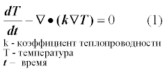
The FVM method is implemented using the heat equation as an example:
So the main steps in implementing FVM:
For the time derivative, we use the standard simplest Euler method. This will be an explicit time scheme where the results from the previous step are taken. And at the first step, they are set as initial conditions.

Using the divergence theorem, the volume integral is converted to the area integral. The meaning is that we replace the integration over the entire internal volume of our element with integration over the surface of this volume only. This formulation is more suitable for the 3D case. For 2D, we will have instead of volume V Is the area of the element, and instead of S is the perimeter of the element. So it turns out that the integral over the area is replaced by the integral over the perimeter. In fact, the degree of the derivative decreases. If for example there was a second derivative, then only ervaya, when was the first - instead of the derivative will be sought peremennaya.Nado just have to remember that we are dealing not with the usual derivative with a divergence.
So the second term in our equation after integration is transformed as follows:


The figure shows Element C and its neighboring elements on the right (E), left (W), top (N) and bottom (S) . Element C has 4 faces indicated by the letters ewns . It is these 4 faces that make up the perimeter of the element and along them integration is performed. For each element, as a result, we obtain a discrete analogue of the original diff equation.
Let’s make a discrete analogue for the element C. To begin with, we need to figure out the integral (3). After all, the integral is in fact the sum, so we replace the integral over the entire surface of the element by the sum of the 4 components of this surface, i.e. 4 faces of the element.

The ewns indices here indicate that an expression or variable is being calculated at the center of the corresponding face.
Now we will collect together the obtained simplifications of the parts of the original diff equation - terms (2) and (4). We get the first stage of approximation:

Now we only need to approximate (4) to the end, since the gradient enters there, we need to convert it to a numerical form. In fact, this sum represents the sum of the heat fluxes through the faces. Our case is simplified for a rectangular grid, because the normal to the face only 1 component remains - either along the x axis or along y.
Let us analyze this process in detail using the example of face e.

Now, substitute the obtained discrete analogues for 4 faces instead of the sum in equation (5):

Equation (7) is the final equation for element C, from it we obtain at each time step a new temperature value (Tnew) in element C.
The figure shows an element C for which the face e is at the boundary and the temperature values on this face are known either as a given temperature or as a given heat flux through the face.

We consider only 2 types of boundary conditions.
Case 2) is the simplest, since it turns out that the face e is not required for sampling (since all the coefficients are Flux = 0) and you can simply skip it.
Now we consider case 1). The discretization of the face e will generally be similar to the one that has already been described. There will be only 2 changes - instead of Te, there will be a known boundary value Tb and instead of the distance DXe there will be DXe / 2. Otherwise, we can consider the value Te as as if it would be a normal neighboring node E. Now we will describe in more detail the term for the boundary element C.

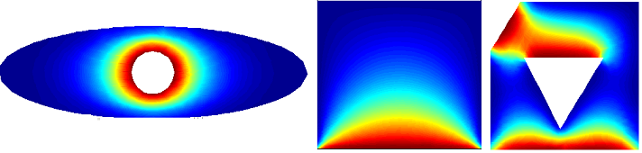
As an example, consider a region divided into 9 elements, a 3 * 3 grid. The following boundary conditions are applied on the first slides: the temperature is T = 0 on 3 sides, the temperature T = 240 is set on the bottom. The boundary conditions with the Flux flow are set on the second line of the slides = 0, above T = 0, below T = 240. For each case, 2 pictures, one with a breakdown of the area 3 * 3 elements, the second 40 * 40.

This is where the advantage of FVM is manifested, where, like in the finite element method, you can represent a region with round borders through the division into triangles or any other polygons. But FVM has one more plus - when switching from triangles to polygons with a large number of sides, absolutely nothing needs to be changed, of course, if the code was written for an arbitrary triangle and not an equilateral one. Moreover, you can use a mixture of different elements — triangles, polygons, squares, etc. without changing the code.
Consider the general case where the vector connecting the centers of the 2 elements does not coincide with the normal vector to the common face of these elements. The calculation of flux flux through the face will now consist of 2 parts. In the first, the orthogonal component will be calculated, and in the second, the so-called cross -diffusion".
The picture shows 2 elements, C is the current element under consideration and F is an adjacent element. We describe the discretization for the face separating these 2 elements. The vector connecting the centers of the elements is DCF. The vector e is a unit vector in the direction of DCF. The vector Sf is directed along the normal to the face, its length is equal to the length of the face.

The calculation scheme looks something like this.

The second term here is cross-diffusion, it will be the greater, the greater the difference between the vectors Ef and Sf, if they coincide, then it is 0.
First we write the orthogonal part (minimum correction method).

In the source, I did not implement the term with cross-diffusion, because the question arose - how to check the correctness of such an implementation. Visually, the comparison of the results of Matlab and mine was no different in the absence of cross-diffusion. Apparently this is due to the fact that Matlab likes triangles close to equilateral, which ultimately makes cross-diffusion = 0. Perhaps later I will return to this issue.
The calculation of the boundary elements is no different from the calculations not at the border, instead of the center of the neighboring element, the center of the face is taken, and, as usual, the temperature at the border is substituted.
In my implementation, it ends up like this:

The check was carried out by comparing the results in Matlab and my implementation. Mesh was used the same, unloaded from Matlab and loaded into the program. For some artifacts-triangles, do not pay attention, this is just an incomprehensible rendering glitch.

The github with sources lies here.
The main version is in the heat2PolyV2 folder. So, what concerns the computing part lies in heat2PolyV2 \ Src \ FiniteVolume \.
At the beginning of the Scene2.cs file there are parameters that can be changed to display in different color schemes, scale, mesh display, etc. The examples themselves are stored in heat2PolyV2 \ bin \ Debug \ Demos \
Unloading from Matlab is simple - you need to open the pde toolbox, open m file (or create it yourself from scratch), go to the Mesh-Export mesh menu, click OK; go to the main Matlab, in the panel there will appear variables - pet matrices, open the savemymesh.m file, execute it, the p.out file will appear, transfer it to the Demos folder.
In the source code, to select an example, you must specify the file name in the line param.file = "p"; (FormParam.cs). Next, you need to apply the boundary conditions - for ready-made examples, you can simply uncomment the corresponding blocks in MainSolver.cs:
The meaning is simple - Matlab divides borders by domain, for example, external and internal. Also, for each domain, the borders are divided into parts (groups) so that you can set conditions on sections of the border separately - for example, to the right or bottom.
It’s possible not to use Matlab at all, but to manually register all the elements (triangles) and their vertices + faces (only for boundary elements)
Finite Volume Method (FVM)
The method is based on dividing the region into disjoint control volumes (elements), nodal points at which the solution is sought. Nodal points are located in the centers of the control volumes. Also, as for the finite difference method, an equation is compiled for each element, and a system of linear equations is obtained. Solving it, we find the values of the
desired variables at the nodal points. For a single element, the equation is obtained by integrating the original diff equation over the element and approximating the integrals.
The term finite volume in the article will often be replaced by the Element, for convenience we will consider them equivalents (the element in this article has nothing to do with the finite element method).
There are 2 different ways to solve the FVM problem:
1) the faces of the control volume coincide with the faces of the element
2) the faces of the control volume pass through the centers of the faces of the elements (into which the region is divided). The desired variables are stored at the vertices of these elements. A control volume is constructed around each vertex. For a non-rectangular grid, this method has 2 more subspecies.
We will use method 1) with control volumes coinciding with the elements into which the region is divided.
Some advantages of FVM:
- preservation of basic quantities throughout the entire region, such as system energy, mass, heat fluxes, etc. Moreover, this condition is fulfilled even for a rough computational grid
- high calculation speed. Many calculated values can be calculated when dividing the area into elements, and there is no need to calculate them at each time step.
- ease of use for tasks with complex geometry and curved borders. Ease of use of different geometric types of elements - triangles, polygons.
The FVM method is implemented using the heat equation as an example:
So the main steps in implementing FVM:
- Translation of a diff equation into a form suitable for FVM - integration over a control volume
- Compilation of a discrete analogue, the choice of a method for translating derivatives and other integrands into discrete form
- Obtaining an equation for each of the control volumes into which the region is divided. Compilation of a system of linear equations and its solution.
Time discretization.
For the time derivative, we use the standard simplest Euler method. This will be an explicit time scheme where the results from the previous step are taken. And at the first step, they are set as initial conditions.
A bit of theory or the first step in implementing FVM
Using the divergence theorem, the volume integral is converted to the area integral. The meaning is that we replace the integration over the entire internal volume of our element with integration over the surface of this volume only. This formulation is more suitable for the 3D case. For 2D, we will have instead of volume V Is the area of the element, and instead of S is the perimeter of the element. So it turns out that the integral over the area is replaced by the integral over the perimeter. In fact, the degree of the derivative decreases. If for example there was a second derivative, then only ervaya, when was the first - instead of the derivative will be sought peremennaya.Nado just have to remember that we are dealing not with the usual derivative with a divergence.
So the second term in our equation after integration is transformed as follows:
FVM on standard rectangular mesh
The figure shows Element C and its neighboring elements on the right (E), left (W), top (N) and bottom (S) . Element C has 4 faces indicated by the letters ewns . It is these 4 faces that make up the perimeter of the element and along them integration is performed. For each element, as a result, we obtain a discrete analogue of the original diff equation.
Let’s make a discrete analogue for the element C. To begin with, we need to figure out the integral (3). After all, the integral is in fact the sum, so we replace the integral over the entire surface of the element by the sum of the 4 components of this surface, i.e. 4 faces of the element.
The ewns indices here indicate that an expression or variable is being calculated at the center of the corresponding face.
Now we will collect together the obtained simplifications of the parts of the original diff equation - terms (2) and (4). We get the first stage of approximation:
Now we only need to approximate (4) to the end, since the gradient enters there, we need to convert it to a numerical form. In fact, this sum represents the sum of the heat fluxes through the faces. Our case is simplified for a rectangular grid, because the normal to the face only 1 component remains - either along the x axis or along y.
Let us analyze this process in detail using the example of face e.
Now, substitute the obtained discrete analogues for 4 faces instead of the sum in equation (5):
Equation (7) is the final equation for element C, from it we obtain at each time step a new temperature value (Tnew) in element C.
Rectangular grid boundary conditions
The figure shows an element C for which the face e is at the boundary and the temperature values on this face are known either as a given temperature or as a given heat flux through the face.
We consider only 2 types of boundary conditions.
- The temperature Tb at the boundary
- The fluxB flow at the boundary is given, we consider only the case when FluxB = 0, i.e. face e will be insulated (Insulated)
Case 2) is the simplest, since it turns out that the face e is not required for sampling (since all the coefficients are Flux = 0) and you can simply skip it.
Now we consider case 1). The discretization of the face e will generally be similar to the one that has already been described. There will be only 2 changes - instead of Te, there will be a known boundary value Tb and instead of the distance DXe there will be DXe / 2. Otherwise, we can consider the value Te as as if it would be a normal neighboring node E. Now we will describe in more detail the term for the boundary element C.
An example of numerical calculations on a rectangular grid
As an example, consider a region divided into 9 elements, a 3 * 3 grid. The following boundary conditions are applied on the first slides: the temperature is T = 0 on 3 sides, the temperature T = 240 is set on the bottom. The boundary conditions with the Flux flow are set on the second line of the slides = 0, above T = 0, below T = 240. For each case, 2 pictures, one with a breakdown of the area 3 * 3 elements, the second 40 * 40.
The calculation code for both cases (in the sources it is called heat2dminimum)
        public void RunPhysic()
        {
            double Tc, Te, Tw, Tn, Ts;
            double FluxC, FluxE, FluxW, FluxN, FluxS;
            double dx = 0;
            double Tb = 240;
            double Tb0 = 0;
            int i, j;
            for (i = 0; i < imax; i++)
                for (j = 0; j < jmax; j++)
                {
                    Tc = T[i, j];
                    dx = dh;
                    if (i == imax - 1) { Te = Tb0; dx = dx / 2; }
                    else
                        Te = T[i + 1, j];
                    FluxE = (-k * FaceArea) / dx;
                    if (i == 0) { Tw = Tb0; dx = dx / 2; }
                    else
                        Tw = T[i - 1, j];
                    FluxW = (-k * FaceArea) / dx;
                    if (j == jmax - 1) { Tn = Tb0; dx = dx / 2; }
                    else
                        Tn = T[i, j + 1];
                    FluxN = (-k * FaceArea) / dx;
                    if (j == 0) { Ts = Tb; dx = dx / 2; }
                    else
                        Ts = T[i, j - 1];
                    FluxS = (-k * FaceArea) / dx;
                    FluxC = FluxE + FluxW + FluxN + FluxS;
                    T[i, j] = Tc + delt * (FluxC * Tc - (FluxE * Te + FluxW * Tw + FluxN * Tn + FluxS * Ts));
                }
        }
        //Insulated
        public void RunPhysic2()
        {
            double Tc, Te, Tw, Tn, Ts;
            double FluxC, FluxE, FluxW, FluxN, FluxS;
            double dx = 0;
            double Tb = 240;
            double Tb0 = 0;
            int i, j;
            for (i = 0; i < imax; i++)
                for (j = 0; j < jmax; j++)
                {
                    Tc = T[i, j];
                    dx = dh;
                    Te = 0; Tw = 0;
                    if (i == imax - 1)
                        FluxE = 0;
                    else
                    {
                        Te = T[i + 1, j];
                        FluxE = (-k * FaceArea) / dx;
                    }
                    if (i == 0)
                        FluxW = 0;
                    else
                    {
                        Tw = T[i - 1, j];
                        FluxW = (-k * FaceArea) / dx;
                    }
                    if (j == jmax - 1) { Tn = Tb0; dx = dx / 2; }
                    else
                        Tn = T[i, j + 1];
                    FluxN = (-k * FaceArea) / dx;
                    if (j == 0) { Ts = Tb; dx = dx / 2; }
                    else
                        Ts = T[i, j - 1];
                    FluxS = (-k * FaceArea) / dx;
                    FluxC = FluxE + FluxW + FluxN + FluxS;
                    T[i, j] = Tc + delt * (FluxC * Tc - (FluxE * Te + FluxW * Tw + FluxN * Tn + FluxS * Ts));
                }
        }
FVM in problems with complex geometry
This is where the advantage of FVM is manifested, where, like in the finite element method, you can represent a region with round borders through the division into triangles or any other polygons. But FVM has one more plus - when switching from triangles to polygons with a large number of sides, absolutely nothing needs to be changed, of course, if the code was written for an arbitrary triangle and not an equilateral one. Moreover, you can use a mixture of different elements — triangles, polygons, squares, etc. without changing the code.
Consider the general case where the vector connecting the centers of the 2 elements does not coincide with the normal vector to the common face of these elements. The calculation of flux flux through the face will now consist of 2 parts. In the first, the orthogonal component will be calculated, and in the second, the so-called cross -diffusion".
The picture shows 2 elements, C is the current element under consideration and F is an adjacent element. We describe the discretization for the face separating these 2 elements. The vector connecting the centers of the elements is DCF. The vector e is a unit vector in the direction of DCF. The vector Sf is directed along the normal to the face, its length is equal to the length of the face.
The calculation scheme looks something like this.
The second term here is cross-diffusion, it will be the greater, the greater the difference between the vectors Ef and Sf, if they coincide, then it is 0.
First we write the orthogonal part (minimum correction method).
In the source, I did not implement the term with cross-diffusion, because the question arose - how to check the correctness of such an implementation. Visually, the comparison of the results of Matlab and mine was no different in the absence of cross-diffusion. Apparently this is due to the fact that Matlab likes triangles close to equilateral, which ultimately makes cross-diffusion = 0. Perhaps later I will return to this issue.
The calculation of the boundary elements is no different from the calculations not at the border, instead of the center of the neighboring element, the center of the face is taken, and, as usual, the temperature at the border is substituted.
In my implementation, it ends up like this:
Calculation code for an arbitrary polygon (in the sources it is called heat2PolyTeach)
        public void Calc()
        {
            double bc, ac;
            double sumflux;
            double[] aa = new double[6];
            double[] bb = new double[6];
            int e;
            for (e = 0; e < elementcount; e++)
            {
                Element elem = elements[e];
                int nf;
                bc = 0;
                ac = 0;
                sumflux = 0;
                for (int nn = 0; nn <6; nn++)
                {
                    aa[nn] = 0;
                    bb[nn] = 0;
                }
                for (nf = 0; nf < elem.vertex.Length; nf++)
                {
                    Face face = elem.faces[nf];
                    Element nb = elem.nbs[nf];
                    if (face.isboundary)
                    {
                        if (face.boundaryType == BoundaryType.BND_CONST)
                        {
                            double flux1;
                            double flux;
                            flux1 = elem.k * (face.area / elem.nodedistances[nf]);
                            Vector2 Sf = face.sf.Clone();
                            Vector2 dCf = elem.cfdistance[nf].Clone();
                            if (Sf * dCf < 0)
                                Sf = -Sf;
                            //1) minimum correction
                            //Vector2 DCF = elem.cndistance[nf].Clone();
                            Vector2 e1 = dCf.GetNormalize();
                            Vector2 EF = (e1 * Sf) * e1;
                            flux = elem.k * (EF.Length() / dCf.Length());
                            ac += flux;
                            bc += flux * face.bndu;
                            bb[nf] = flux;
                        }
                        else if (face.boundaryType == BoundaryType.BND_INSULATED)
                        {
                            double flux;
                            flux = 0;
                            ac += flux;
                            bc += flux * face.bndu;
                            bb[nf] = flux;
                        }
                    }
                    else
                    {
                        double flux1;
                        double flux;
                        flux1 = -elem.k * (face.area / elem.nodedistances[nf]);
                        Vector2 Sf = face.sf.Clone();
                        Vector2 dCf = elem.cfdistance[nf].Clone();
                        if (Sf * dCf < 0)
                            Sf = -Sf;
                        Vector2 DCF = elem.cndistance[nf].Clone();
                        Vector2 e1 = DCF.GetNormalize();
                        //corrected flux
                        //1) minimum correction
                        Vector2 EF = (e1 * Sf) * e1;
                        flux = -elem.k * (EF.Length() / DCF.Length());
                        sumflux += flux * nb.u;
                        ac += -flux;
                        aa[nf] = -flux;
                    }
                }
                elem.u = elem.u + delt * (bc - sumflux - ac * elem.u);
            }
        }
Examples and verification of results
The check was carried out by comparing the results in Matlab and my implementation. Mesh was used the same, unloaded from Matlab and loaded into the program. For some artifacts-triangles, do not pay attention, this is just an incomprehensible rendering glitch.
Description of the source structure
The github with sources lies here.
The main version is in the heat2PolyV2 folder. So, what concerns the computing part lies in heat2PolyV2 \ Src \ FiniteVolume \.
At the beginning of the Scene2.cs file there are parameters that can be changed to display in different color schemes, scale, mesh display, etc. The examples themselves are stored in heat2PolyV2 \ bin \ Debug \ Demos \
Unloading from Matlab is simple - you need to open the pde toolbox, open m file (or create it yourself from scratch), go to the Mesh-Export mesh menu, click OK; go to the main Matlab, in the panel there will appear variables - pet matrices, open the savemymesh.m file, execute it, the p.out file will appear, transfer it to the Demos folder.
In the source code, to select an example, you must specify the file name in the line param.file = "p"; (FormParam.cs). Next, you need to apply the boundary conditions - for ready-made examples, you can simply uncomment the corresponding blocks in MainSolver.cs:
  //p.out
  public void SetPeriodicBoundary()
The meaning is simple - Matlab divides borders by domain, for example, external and internal. Also, for each domain, the borders are divided into parts (groups) so that you can set conditions on sections of the border separately - for example, to the right or bottom.
It’s possible not to use Matlab at all, but to manually register all the elements (triangles) and their vertices + faces (only for boundary elements)
Description of the .out file structure
The file is divided into sections - ## Points (vertices), ## Triangle (triangles) and ## Boundary (faces - only those that are on the border)
## Points - coordinates of points, the first line is x, the second is y.
## Triangle - triangles, the first line is the index of the 1st vertex in the ## Points array, the 2nd and 3rd lines are the indices of the 2nd and 3rd vertices of the triangle.
## Boundary - faces, the first row is the index of the 1st vertex of the face, the 2nd is the index of the second vertex, the fifth row is the group, the sixth is the domain
## Points - coordinates of points, the first line is x, the second is y.
## Triangle - triangles, the first line is the index of the 1st vertex in the ## Points array, the 2nd and 3rd lines are the indices of the 2nd and 3rd vertices of the triangle.
## Boundary - faces, the first row is the index of the 1st vertex of the face, the 2nd is the index of the second vertex, the fifth row is the group, the sixth is the domain
Description of source folders
Sources are written in Visual Studio 2010 c #. Used Matlab R2012a.
Github with source
Github with source
- heat2PolyV2 - final version
- other \ heat2Utrianglestatic - implemented an example from the book p346 versteeg_h malalasekra_w_ An_introduction_to_computational_fluid ...
- other \ water2dV2 - an attempt to solve the Navier-Stokes equations partially using FiniteVolume
- matlab - m example files pde toolbox + savemymesh.m which unloads the finished .out file for heat2PolyV2
List of books on the topic
- Versteeg HK Malalasek Introduction to computational fluid dynamics The finite volume method - there is already a second edition
- F.Moukalled L.Mangani M.Darwish The finite volume method in computational fluid dynamics 2016 - released recently (almost yesterday :)
- Patankar S. — Numerical methods for solving heat transfer problems and fluid dynamics — Energoatomizdat (1984)
- Patankar S.V.-Numerical solution of the problems of heat conduction and convective heat transfer during flow in channels-MPEI (2003)
- Computational methods for fluid dynamics Ferziger JH Peric 2001 - although not directly related to FVM, but a lot of useful