Online Algorithms in High-Frequency Trading: Problems of Competition / ITI Capital Blog

High Frequency Trading High-frequency trading, HFT-trading] today has a great influence on modern financial markets. Even 20 years ago, most of the trading took place on exchanges, for example, on the New York Stock Exchange, where people dressed in colorful costumes actively gestured and shouted their offers to buy or sell securities. Today, trading is usually carried out using electronic servers in data centers, where computers exchange offers to buy and sell by sending messages over the network. This transition from trading in the exchange’s operational building to electronic platforms was especially beneficial for HFT companies that invested a lot of money in the necessary infrastructure for trading.

Despite the fact that the place and participants of the trade outwardly changed greatly, the goal of traders - both electronic and ordinary - remained unchanged - to acquire an asset from one company / trader and sell it to another company / trader at a higher price. The main difference between a traditional trader and an HFT trader is that the latter can trade faster and more often, and the portfolio holding time for such a trader is very low. One operation of the standard HFT algorithm takes a fraction of a millisecond, which traditional traders cannot compare with, since a person blinks about once every 300 milliseconds. As HFT algorithms compete with each other, they face two problems:

• Each microsecond they process a large amount of data;
• They need to be able to react very quickly based on these data, because the profit that they can extract from the signals they receive decreases very quickly.

Online algorithms are a common class of algorithms that can be used in HFT trading. In such algorithms, new input variables arrive sequentially. After processing each new input variable, the algorithm must make a specific decision, for example, whether to submit a purchase / sale request. This is the main difference between online algorithms and offline algorithms, in which it is believed that all input data is available at the time of decision making. Most of the tasks of practical optimization in such areas as computer science and methods of operations research are precisely online problems [1].

In addition to solving online problems, HFT algorithms also need to respond extremely quickly to market changes. To respond to the situation faster, an online trading algorithm must work efficiently with memory. Storing a large amount of data reduces the speed of any computer, so it is important that the algorithm uses a minimum amount of data and parameters that can be stored in high-speed memory, for example, in the cache of the first level (L1). In addition, this set of parameters should reflect the current state of the market and be updated as new variables arrive in real time. Thus, the smaller the number of parameters that need to be stored in memory, and the less calculations need to be performed for each of these parameters, the faster the algorithm will be able to respond to market changes.

Considering the speed requirements and the online nature of HFT trading tasks, the class of single-pass algorithms can be successfully applied in HFT trading. At each selected point in time, these algorithms receive one data element at the input and use it in order to update the set of available parameters. After the update, one of the data elements is discarded, and thus only the updated parameters are stored in memory.

When developing the HFT algorithm, three problems can arise. The first is to evaluate the moving average liquidity: solving this problem can help the HFT algorithm determine the size of the order, which is most likely to be executed successfully on this electronic exchange. The second is to evaluate moving volatility: solving this problem helps determine the short-term risk for a particular position. The third problem is based on the concept of linear regression, which can be used in pair trading of related assets.
Each of these problems can be easily solved using a single-pass online algorithm. This article describes how the back-testing of a single-pass algorithm was carried out on the basis of data taken from the book of limit orders for highly liquid exchange-traded investment funds, and gives recommendations for regulating the operation of these algorithms in practice.

Online Algorithms in HFT Trading

One of the advantages of HFT-traders over other market participants is the speed of reaction. HFT companies can track any movement in the market - that is, the information contained in the book of limit orders - and based on it make an appropriate decision within a few microseconds. Although the actions of some HFT algorithms may be based on data from a source located outside the market (for example, when analyzing news reports, measuring temperature or evaluating market trends), most make decisions solely on the basis of messages received directly from the market. According to some estimates, quotes on the New York Stock Exchange are updated approximately 215,000 times per second [2]. The main task of HFT algorithms is to process the received data in such a way that it is possible to make the right decisions, for example, when to put a position or reduce risk. The examples in this article take into account that HFT algorithms can see any price update of the best bid or ask, including data on their sizes. Such a subclass of data contained in the book of limit orders is often called information from the book of orders of the first level (Level-1).

This article details three examples of online algorithms, each of which is intended for use in HFT trading:

• Online algorithm for calculating the mathematical expectation . Designed to find a parameter based on which you can predict the available liquidity, calculated as the sum of the sizes of the best bid and ask, over a fixed period of time in the future. Determining this value can help estimate the size of the application, which is most likely to be executed at the best price, taking into account this delay.
• Online algorithm for calculating variance . Designed to find a parameter on the basis of which it is possible to predict the realized volatility over a fixed period of time in the future. Determining this value can help assess the short-term risk of stockpiling.
• Online algorithm for calculating the regression coefficient . Designed to find a parameter based on which you can predict the expected profit from holding long and short positions of a pair of related assets. The determination of this value can help in creating a signal that is generated when the long and short positions are most likely to be profitable.

In each of the three cases, the algorithm contains a single parameter, “alpha,” which controls the speed at which unnecessary information is discarded. In Figure 1, blue indicates the approximate change in liquidity (the sum of the bid and ask sizes). Red and green indicate the change in the liquidity parameter with the values ​​of the parameter alpha equal to 0.9 and 0.99, respectively. Please note that as the alpha approaches one, the signal level becomes more uniform and more accurately reflects the trend in the source data.



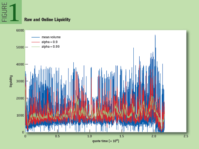
Fig. 1: Uncleaned and online liquidity

Figure 2 shows the change in volatility for different values ​​of the alpha parameter in real time. Please note that, as in the previous case, with an increase in alpha, the graph curve becomes smoother. A higher value of "alpha" gives a more even signal, but a high load of past data causes a lag behind the current trend. As will be shown later, the selection of a suitable value of "alpha" will either give a more even signal, or reduce the lag from the trend.



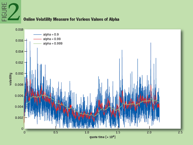
Fig. 2: Measure online volatility for different alpha values

To show how the online regression algorithm works, we looked at time series made up of average stock prices of SPY and SSO - two related exchange-traded investment funds (SSO is the same SPY, but its borrowed funds are twice as large). As shown in Figure 3, the relationship between these two assets during the course of their change during the day is close to linear. Figure 4 shows the change in mathematical expectation and free term for the two alpha values.



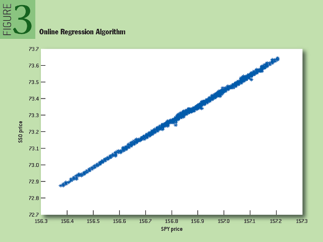
Fig. 3: Online Regression Algorithm



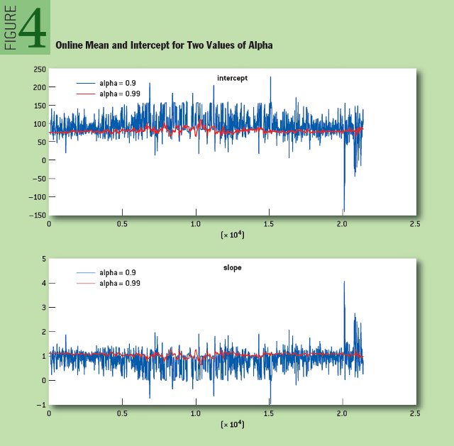
Fig. 4: Change in mathematical expectation and free term for two alpha values

Single pass algorithms

As the name implies, a one-pass algorithm reads the input variable exactly once and then discards it. This type of algorithm allocates memory efficiently since it saves a minimal amount of data. This section provides three important examples of single-pass algorithms: exponentially moving average, exponentially weighted variance, and exponentially weighted regression. The next section will discuss the application of these algorithms in HFT trading.

To begin with, we briefly consider the concept of a simple moving average for a given time series. It is an estimate of the mathematical expectation for a time series with a “sliding” window of constant size. In the financial sector, this estimate is often used to determine the price trend, in particular, when comparing two values ​​of a simple moving average - in the case of a "long" window and in the case of a "short" window. As an application, you can also consider a situation where the average trading volume in the last five minutes helps to predict the volume of trade in the next minute. Unlike an exponential moving average, a simple moving average cannot be determined using a single-pass algorithm.

Let (X _t ) _t = X ₀ , X₁ , X ₂ , ... is a sequence of received input variables.

For each individual moment of time t, we need to predict the value of the next variable X _{t + 1} . For M> 0 and t ≥ M, a simple moving average with a window of size M is defined as the mathematical expectation of the last M observations for the time series (X _t ) _t , that is 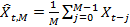. The moving average can also be calculated by the following recursion

. (1)

Although this is an online algorithm, nevertheless, it is not single-pass, because it has to process each input element twice: when it needs to be taken into account when calculating the moving average and when it needs to be excluded from the estimate. Such an algorithm is called a two-pass algorithm and requires storage in memory of an entire array of size M.

Example 1: One-pass exponentially weighted average algorithm

Unlike the usual average 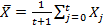, the exponentially weighted average determines the exponentially decreasing values ​​of the weighting coefficients of previous observations: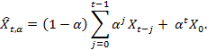



Here, α is the weighted parameter that is selected by the user and must satisfy the condition 0 <α ≤ 1. Due to the fact that an important role is played by the exponentially weighted average the most recent input parameters, compared to earlier data elements, are often considered a fairly accurate approximation of a simple moving average.

Unlike a simple moving average, an exponentially weighted average takes into account all previous data, not just the last M observations. Moreover, if we further compare the simple moving average and the exponentially weighted average, in Figure 5 we can see how many data elements receive 80%, 90%, 95%, 99%, and 99.9% of the weight function depending on α during the evaluation. For example, if α = 0.95, then the last M = 90 received data elements make up 99% of the estimated value. It should be noted that if the time series (Xt) t have very “heavy tails”, then the exponentially smoothed average can consist mainly of extreme observations, while the moving average less often depends on extreme observations, since they are ultimately excluded from the observation window.



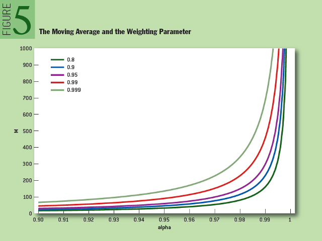
Fig. 5: Moving average and weight parameter.

The reason for choosing an exponentially moving average instead of a simple moving average for use in the HFT algorithm is that it can be determined using a single-pass algorithm, first mentioned by R.G. Brown (1956) [3].

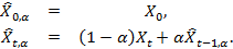. (2)

This formula also indicates that, using parameter α, weights of the latest observations can be adjusted by comparing them with the previous ones.

Example 2: Single Pass Exponentially Weighted Variance Algorithm

The exponential smoothing described in the previous section allows us to estimate the moving average for time series. In finance, time series volatility often plays an important role. In other words, volatility should reflect the frequency of fluctuations of time series relative to their average level. There is no unambiguous definition of volatility in the financial theory of HFT trading. In this section, volatility is considered as the standard deviation (square root of variance) of a data element for time series (X _t ) _t . As in the case of the exponentially weighted moving average from the previous section, you can develop a one-pass online algorithm that will evaluate the volatility for time series based on the scheme of exponentially weighted coefficients.

The variance of a random variable is determined by the formula Var (X) = E [X - E [X]) ² ]. In order to estimate the exponentially weighted variance of time series, it is first necessary to estimate two parameters - the mathematical expectation E [X] and the variance:



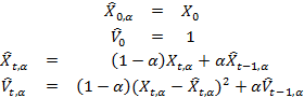
The standard deviation of each next control point X _{t + 1} is estimated as. In this example, the input parameter α ∈ (0,1) is also selected by the user and determines the values ​​of the weight coefficients of the past data, which are compared with the last of the received input data. In this case, we take the initial value of the statistical estimate equal to 1 - it [rating], generally speaking, can take any value. Another way is to introduce a trial period during which time series are monitored and use the standard deviation estimate for time series in this “test” window as an initial estimate. Of course, a similar method can also be used to determine an estimate of an exponentially weighted average.

Example 3: One-pass exponentially weighted linear regression algorithm

The latest example is a one-pass online algorithm based on an exponentially weighted linear regression model. This model is similar to the conventional linear regression model, but in contrast, it focuses more attention (in accordance with exponential weighting) on ​​recent observations than on earlier ones. As already shown, such regression methods play an important role in HFT strategies and help to determine the relationship between various assets, in particular, they can be used in pair trading strategies.

In our model, we consider two-dimensional time series (X _t , Y _t ) _t and assume that the variables X and Y are connected by a linear relation, which also includes a random error ε _twith zero expectation, ie:

. (3) The

variable Y is called the response variable, and the variable X is called the explanatory variable. For simplicity, suppose we have one explanatory variable, although it is not so difficult to generalize to several explanatory variables. With the standard approach to determining linear regression using the offline algorithm, the parameters β ₀ and β _{1 are} selected after all the observations. The data elements of each individual observation are written in a separate vector Y = (Y ₀ , Y ₁ , ..., Y _t ) ^T or a matrix.



A column of units in the matrix X corresponds to the free term in equation 3. If we write the parameters β ₀and β ₁ in the form of a vector β = (β ₀ , β ₁ ) ^T , then the relationship between Y and X can be compactly written in matrix form:

Y = Xβ + ε

where ε is a vector of stochastic errors, each of which has zero mathematical expectation.

The most common approach to estimating the parameter β is to use the standard least-squares method, that is, β is chosen so that the sum of the squares of the residual terms is minimal. The solution to this minimization problem will be .

As in the estimation of mathematical expectation and variance, later observations should play an important role in estimating the parameter β. In addition, a one-pass algorithm for finding β values ​​is needed for calculations.

Next, we consider a recursive method that sequentially updates the values ​​of the vector β and minimizes the expression:



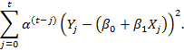
Recall that the parameter must be on the interval (0,1) and selected by the user. The parameters β _{0 and} β ₁ estimates using the method of weighted least squares can be calculated using an effective single-pass online algorithm. At each step of the algorithm, a 2 × 2 matrix M _t and a vector V _t2 × 1 dimensions must be stored in memory and updated as new data are obtained in accordance with the following recursive expressions:



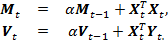
As for the estimate of mathematical expectation and variance, for them, the recursion variables can be initialized in the trial period. As a result, by time t, the best estimate of β will be calculated by the formula . In the literature, this method is called the recursive least squares method with exponential forgetting [2].

Alpha score

How to determine the optimal value of "alpha", the only parameter used in each of the above models of online algorithms? Our approach in each of the three models was to determine the response function, the value of which we want to predict, and minimize the square of the difference between the response ri and our parameter f _i :



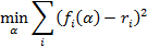
This method allows us to determine the optimal value of "alpha" based on historical time series. Another approach is to evaluate the optimal value of "alpha", which is also carried out in real time. However, it requires more work and is beyond the scope of this article.

Now, let’s take a closer look at the estimates of online algorithms described in more detail and evaluate the optimal alpha value on a specific data set.
1. The average liquidity rating is calculated by the formula:



where the index i denotes the point in time when the quote was set. The response function is defined as liquidity, which is observed after ten seconds:



where the term b _si (10) is the size of the bid ten seconds after setting the i-th quote. After optimizing for the alpha parameter, it was shown that the optimal alpha value for our data is 0.97. It is presented in Fig. 6 in the form of a scattering diagram for the desired parameter and response function:



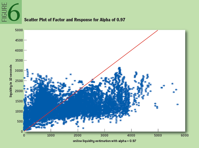
Fig. 6: Scatter plot for the desired parameter and response function for the alpha value of 0.97

2. The volatility score is determined by the formulas:







where the index i denotes the current time in seconds. The value of the response is defined as the realized volatility in the last minute:



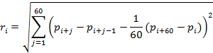
As in the previous case, as a result of enumerating the values ​​of the "alpha" parameter, the optimal value for our data set was 0.985. Figure 7 shows the scattering diagram for the required parameter and the response function:



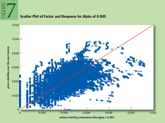
Fig. 7: The scatter chart and response function for alpha is 0.985

3. The regression estimate for pair trading is found by the formulas:









where the index i denotes the time when the quote was set. The parameter indicates the value of SPY stocks compared to SSO stocks, that is, if their difference is positive, then SPY stocks are relatively cheaper, and holding a long position on SPY is likely to be profitable.

The response function is defined as the profit received in the last minute from the transaction, which consists of holding a long position per SPY share and a short position on β SSO shares:



where is the value of the SPY share 60 seconds after the value is set . The response r _i indicates the profitability of the following strategy for holding a long and short position: “Buy one SPY share and sell β SSO shares at time i, after 60 seconds close the position.”

On the studied data set, the optimum value was "alpha", equal to 0.996. Figure 8 shows the scattering diagram for the required parameter and the response function:



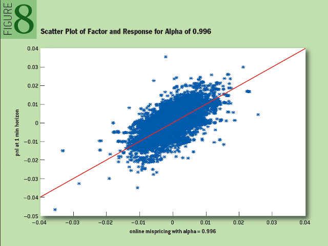
Fig. 8: Scatter plot and response function for alpha 0.996

Conclusion

Single-pass online algorithms are an effective tool in HFT trading, where they have to process large amounts of data every microsecond and make decisions based on them very quickly. This article examined three problems that HFT algorithms face: an estimate of the moving average liquidity needed to determine the size of an order, which is most likely to be executed successfully on a particular electronic exchange; assessment of the moving volatility necessary to calculate the short-term risk of a particular transaction; sliding linear regression, which can be used in pair trading of related assets. Single-pass online algorithms can play a key role in solving these problems.

Another important factor for HFT-traders, which we often write about on the Habré blog, is the speed of work. One of the commonly used technologies to increase the speed of obtaining and processing data is direct access to the exchange , which is organized using various protocols for transferring financial information. We considered direct access technology in this article , and wrote about data transfer protocols here ( one , two , three ).

Notes:

1. Albres S. 2003. Online Algorithms: Analysis. Math Programming 97 (1-2): 3-26.
2. Кларк К. 2011. Улучшение скорости и прозрачности рыночных данных. Биржи. whatheheckaboom.wordpress.com/2013/10/20/acm-articles-on-hft-technology-and-algorithms, www.utpplan.com .
3. Браун Р. Г. 1956. Экспоненциальное сглаживание для прогнозирования спроса. Arthur D. Little Inc., с. 15.
4. Астром А., Уиттенмарк Б. 1994. Адаптивное управление, второе издание. Addison Wesley.

About the Authors:

Jacob Loveless (Jacob Loveless) - Executive Director of Lucera and former head of the department of high-frequency trading in the Cantor Fitzgerald. Over the past ten years, Mr. Loveless has managed to try his hand at electronic trading in virtually every asset in various HFT companies and on various exchanges. Before starting a career in the financial sector, Mr. Loveless was a special contractor for the US Department of Defense, specializing in heuristic analysis of secret data. Prior to that, he was also CTO and founder of Data Scientific. Founder of distributed systems analysis.

Sasha Stoikov- Senior Fellow at Cornell Financial Engineering Manhattan School (CFEM) and former Vice President of High Frequency Trading at Cantor Fitzgerald. He worked as a consultant at the Galleon Group and Morgan Stanley, and also lectured at the Institute. Courant at New York University and the Department of Organization of Production and Operations Research at Columbia University. He received a Ph.D. at the University of Texas and a bachelor's degree at the Massachusetts Institute of Technology.

Rolf Waeber- A specialist in quantitative analysis at Lucera, in the past he was engaged in quantitative research in the high-frequency trading department of Cantor Fitzgerald. He took part in liquidity risk management research as part of the development of Basel II / III documents at the German Federal Bank. In 2013, Rolf received his Ph.D. in operations research and information engineering from Cornell University. In addition, he received bachelor's and master's degrees in mathematics at the Zurich High School of Technology, Switzerland.