Visualization of static and dynamic networks on R, part 4
- Transfer
- Tutorial
In the first part :
In the second part : colors and fonts in the graphs of R.
In the third part: parameters of graphs, vertices and edges.
In this part: network hosting.
Network locations are algorithms that return the coordinates of each vertex of a graph.
To study the placements, create a slightly larger graph of 80 vertices. We use the barabasi.game function, which generates a simple graph starting from one vertex and increasing vertices and edges depending on the given level of preferred attachment (how many more new objects will prefer to establish communication with more popular vertices on the network).

You can specify the placement in the build function:

Or calculate the coordinates of the vertices in advance:


This placement is just an example; it is not very useful. Fortunately, igraph has a set of built-in placements, including the following:


Fruchtermann-Reingold is one of the most commonly used force placement algorithms.
Power placement involves creating a beautiful graph with edges of the same length and the minimum possible number of intersections. They represent the graph in the form of a physical system. Vertices are electrically charged particles that repel each other with excessive approximation. The ribs behave like springs attracting connected vertices closer to each other. As a result, the vertices are evenly distributed over the graph area, and the placement is intuitive in the sense that the vertices with a large number of links are closer to each other. The disadvantage of these algorithms is that they are rather slow, and therefore rarely used on graphs with more than 1000 vertices.
Here are a few parameters that can be set for this placement:
You can also use the “weight” parameter, which increases the attractive forces between the vertices connected by heavier ribs.
You will notice that the placement is not strictly defined - different launches lead to slightly different configurations. Saving Placement
Accommodation is

Another popular force placement algorithm showing good results for connected graphs is Kamada-Kawai. Like Fruchtermann-Reingold, his goal is to minimize energy in the spring system. Igraph also contains a spring-based layout called

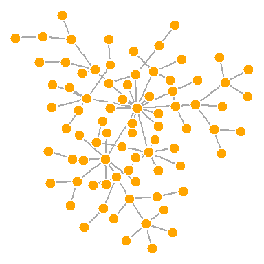
The LGL (Large Graph Layout) algorithm is designed for large connected graphs. It also allows you to specify the root - the vertex, which will be located in the center of the placement.
By default, the coordinates of the graphs are scaled to the interval [-1.1] in both x and y. This can be changed using the parameter

By default, igraph uses placement
Let's look at the placements available in igraph:

- network visualization: why? how?
- visualization options
- best practices - aesthetics and performance
- data formats and preparation
- description of the data sets used in the examples
- getting started with igraph
In the second part : colors and fonts in the graphs of R.
In the third part: parameters of graphs, vertices and edges.
In this part: network hosting.
Network placements
Network locations are algorithms that return the coordinates of each vertex of a graph.
To study the placements, create a slightly larger graph of 80 vertices. We use the barabasi.game function, which generates a simple graph starting from one vertex and increasing vertices and edges depending on the given level of preferred attachment (how many more new objects will prefer to establish communication with more popular vertices on the network).
net.bg <- barabasi.game(80)
V(net.bg)$frame.color <- "white"
V(net.bg)$color <- "orange"
V(net.bg)$label <- ""
V(net.bg)$size <- 10
E(net.bg)$arrow.mode <- 0
plot(net.bg)
You can specify the placement in the build function:
plot(net.bg, layout=layout.random)
Or calculate the coordinates of the vertices in advance:
l <- layout.circle(net.bg)
plot(net.bg, layout=l)
l- matrix of x- and y-coordinates (N x 2) for N vertices of the graph. You can easily set them yourself:l <- matrix(c(1:vcount(net.bg), c(1, vcount(net.bg):2)), vcount(net.bg), 2)
plot(net.bg, layout=l)
This placement is just an example; it is not very useful. Fortunately, igraph has a set of built-in placements, including the following:
# Случайно расположенные вершины
l <- layout.random(net.bg)
plot(net.bg, layout=l)
# Размещение по кругу
l <- layout.circle(net.bg)
plot(net.bg, layout=l)
# Размещение в виде 3D-сферы
l <- layout.sphere(net.bg)
plot(net.bg, layout=l)
Fruchtermann-Reingold is one of the most commonly used force placement algorithms.
Power placement involves creating a beautiful graph with edges of the same length and the minimum possible number of intersections. They represent the graph in the form of a physical system. Vertices are electrically charged particles that repel each other with excessive approximation. The ribs behave like springs attracting connected vertices closer to each other. As a result, the vertices are evenly distributed over the graph area, and the placement is intuitive in the sense that the vertices with a large number of links are closer to each other. The disadvantage of these algorithms is that they are rather slow, and therefore rarely used on graphs with more than 1000 vertices.
Here are a few parameters that can be set for this placement:
area(by default - the square of the number of vertices) and repulserad(suppression radius for repulsion - area times the number of vertices). Both parameters affect the layout of the chart - change them until you are satisfied with the result. You can also use the “weight” parameter, which increases the attractive forces between the vertices connected by heavier ribs.
You will notice that the placement is not strictly defined - different launches lead to slightly different configurations. Saving Placement
lallows you to get the same result many times, which can be useful if you need to build a graph change in time or different relationships - and you need to leave the vertices at the same places in several graphs. Accommodation is
fruchterman.reingold.gridsimilar fruchterman.reingoldbut faster.l <- layout.fruchterman.reingold(net.bg, repulserad=vcount(net.bg)^3,
area=vcount(net.bg)^2.4)
par(mfrow=c(1,2), mar=c(0,0,0,0)) # построить два графика - 1 строка, 2 столбца
plot(net.bg, layout=layout.fruchterman.reingold)
plot(net.bg, layout=l)
dev.off() # выключить графику, чтобы очистить конфигурацию.
Another popular force placement algorithm showing good results for connected graphs is Kamada-Kawai. Like Fruchtermann-Reingold, his goal is to minimize energy in the spring system. Igraph also contains a spring-based layout called
layout.spring().l <- layout.kamada.kawai(net.bg)
plot(net.bg, layout=l)
l <- layout.spring(net.bg, mass=.5)
plot(net.bg, layout=l)
The LGL (Large Graph Layout) algorithm is designed for large connected graphs. It also allows you to specify the root - the vertex, which will be located in the center of the placement.
plot(net.bg, layout=layout.lgl)
By default, the coordinates of the graphs are scaled to the interval [-1.1] in both x and y. This can be changed using the parameter
rescale=FALSEand manually scale the graph by multiplying the coordinates by a number. The function layout.normallows you to normalize the chart at the desired boundaries.l <- layout.fruchterman.reingold(net.bg)
l <- layout.norm(l, ymin=-1, ymax=1, xmin=-1, xmax=1)
par(mfrow=c(2,2), mar=c(0,0,0,0))
plot(net.bg, rescale=F, layout=l*0.4)
plot(net.bg, rescale=F, layout=l*0.6)
plot(net.bg, rescale=F, layout=l*0.8)
plot(net.bg, rescale=F, layout=l*1.0)
dev.off()
By default, igraph uses placement
layout.auto. It automatically selects the necessary placement algorithm based on the properties of the graph (size and connectivity). Let's look at the placements available in igraph:
layouts <- grep("^layout\\.", ls("package:igraph"), value=TRUE)
# Убрать размещения, не подходящие для нашего графа.
layouts <- layouts[!grepl("bipartite|merge|norm|sugiyama", layouts)]
par(mfrow=c(3,3))
for (layout in layouts) {
  print(layout)
  l <- do.call(layout, list(net))
  plot(net, edge.arrow.mode=0, layout=l, main=layout) }
dev.off()