10+ Tips for Writing Quick Code in Mathematica
- Transfer
- Tutorial
Translation of Jon McLoone's post " 10 Tips for Writing Fast Mathematica Code ". Many
thanks to Kirill Guzenko KirillGuzenko for help with the translation.
A post by John MacLoon talks about common techniques for speeding up code written in the Wolfram Language. For those who are interested in this issue, we recommend that you familiarize yourself with the video “Code Optimization in Wolfram Mathematica”, from which you will learn in detail and with many interesting examples about code optimization techniques, as discussed in the article (but in more detail), and others.
When people tell me that Mathematica is not fast enough, I usually ask you to look at the code and often find that the problem is not Mathematica's performance , but its not optimal use. I would like to share a list of the things that I pay attention to first of all when trying to optimize the code in Mathematica .
The most common mistake that I notice when I deal with slow code is a task of too high accuracy for this task. Yes, inappropriate use of exact symbolic arithmetic is the most common case.
Most computing software systems have no such thing as exact arithmetic - for them 1/3 is the same as 0.33333333333333. This difference can play a big role when you are faced with complex and unstable tasks, however, for most tasks, floating-point numbers are quite satisfactory, and what is important - calculations with them are much faster. In Mathematicaany number with a point and with less than 16 digits is automatically processed with machine precision, therefore you should always use a decimal point if speed is more important than accuracy in this task (for example, enter a third as 1./3.). Here is a simple example where working with floating-point numbers is almost 50.6 times faster than working with exact numbers, which will only then be converted to floating-point numbers. And in this case the same result is obtained.




The same can be said for symbolic calculations. If the symbolic form of the answer is not important for you and stability does not play a special role in this task, then try to switch to the form of a floating-point number as soon as possible. For example, solving this polynomial equation in symbolic form, before substituting the values, Mathematica builds an intermediate symbolic solution on five pages.


But if you first perform the substitution, Solve will use much faster numerical methods.


When working with data lists, you should be consistent in using real numbers. Just one exact value in the data set will translate it into a more flexible, but less efficient form.


The Compile function accepts Mathematica code and allows you to pre-set the types (real, complex, etc.) and structures (value, list, matrix, etc.) of the input arguments. This deprives part of the flexibility of the Mathematica language , but eliminates the need to worry about “What if the argument is in symbolic form?” And other similar things. Mathematica can optimize the program and create byte code to run it on its virtual machine (compilation in C is also possible - see below). Not everything can be compiled, and very simple code may not get any benefits, but complex and low-level computing code can get really great acceleration.
Here is an example:


Using Compile instead of Function gives acceleration more than 80 times.



But we can go further by telling Compile about the possibility of parallelizing this code, getting even better results.



On my dual-core machine, I got the result 150 times faster than in the original case; the increase in speed will be even more noticeable with a large number of cores.
However, keep in mind that many functions in Mathematica , such as Table , Plot , NIntegrate, and some others automatically compile their arguments, so you won’t see any improvements when using Compile for your code.
In addition, if your code compiles, then you can also use the CompilationTarget -> “C” option to generate C code, which will automatically call the C compiler to compile into a DLL and send a link to it in Mathematica . We have additional costs at the compilation stage, but the DLL is executed directly in the processor, and not in the Mathematica virtual machine , so the results can be even faster (in our case, 450 times faster than the original code).



Mathematica has many features. More than an ordinary person can learn in one sitting (the latest version of Mathematica 10.2 already contains more than 5000 functions). So it is not surprising that I often see code where someone implements some operations, not knowing that Mathematica already knows how to implement them. And this is not only a waste of time on the invention of a bicycle; our guys worked hard, creating and most efficiently implementing the best algorithms for various types of input data, so the built-in functions work really fast.
If you find something similar, but not quite, then you should check the parameters and optional arguments - they often generalize functions and cover many special and more distant applications.
Here is an example. If I have a list of a million 2x2 matrices that I want to turn into a list of a million one-dimensional lists of 4 elements, then in theory the easiest way would be to use Map on the Flatten function applied to the list.



But Flatten knows how to solve this problem herself, if you indicate that levels 2 and 3 of the data structure should be combined, and level 1 should not be affected. Indication of such details may be somewhat inconvenient, however, using only one Flatten , our code will be executed 4 times faster than in the case when we will reinvent the features built into the function.


So do not forget to look in the help before entering any of your functionality.
Mathematica forgives some kinds of errors in the code, and everything will work quietly if you suddenly forgot to initialize the variable at the right time, and you do not need to worry about recursion or unexpected data types. And this is great when you just need to quickly get an answer. However, such an error code will not allow you to get the best solution.
Workbench helps in several ways. Firstly, it allows you to better debug and organize large projects, and when everything is clear and organized, it is much easier to write good code. But the key feature in this context is the profiler, which allows you to see which lines of code are used at certain points in time, how many times they were called.
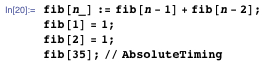
Let us consider as an example a similar, terribly non-optimal (from the point of view of calculations) method of obtaining Fibonacci numbers . If you did not think about the consequences of double recursion, then you will probably be somewhat surprised at the 22nd seconds to evaluate fib [35] (approximately the same amount of time will be required for the built-in function to calculate all 208 987 639 digits of Fibonacci [1,000,000,000] [see paragraph 3] )

Coder execution in Profiler shows the reason. The main rule is called 9,227,464 times, and fib [1] is requested 18,454,929 times.
Seeing the code as it really is can be a real revelation.
This is good advice for programming in any language. Here's how it can be implemented in Mathematica :

It saves the result of calling f for any argument, so if the function is called for an argument that has already been called, then Mathematica will not need to calculate it again. Here we give the memory, in return, getting the speed, and, of course, if the number of possible arguments to the function is huge, and the probability of calling the function again with the same argument is very small, then you should not do this. But if the many possible arguments are small, then this can really help. This code saves the program that I used to illustrate tip 3. You need to replace the first rule with this:

And the code starts to work incomparably fast, and for calculating fib [35] the main rule should be called only 33 times. Storing the previous results prevents the need to repeatedly descend to fib [1] repeatedly .
A growing number of operations in Mathematica are automatically distributed to local kernels (especially problems of linear algebra, image processing, statistics), and, as we have already seen, can be implemented on request through Compile . But for other operations that you want to parallelize on remote equipment, you can use the built-in constructs to parallelize.
There is a set of tools for this, however, in the case of fundamentally mono-threaded tasks, the use of ParallelTable , ParallelMap and ParallelTry alonemay increase computing time. Each of the functions automatically solves the tasks of communication, management and collection of results. There are some additional costs in sending the task and getting the result, that is, getting time gain in one, we lose time in the other. Mathematica comes with a certain maximum number of processing cores available (license dependent), and you can scale them with Mathematica grid if you have access to additional cores. In this example, ParallelTable gives me double performance as it runs on my dual core machine. A larger number of processors will give a larger increase.


Everything Mathematica Can Domay be parallelized. For example, you can send sets of parallel tasks to remote devices, each of which compiles and runs in C or on the GPU.
Using the GPU, some tasks can be solved in parallel much faster. Apart from the case when you need functions that are already optimized for CUDA to solve your tasks, you need to do a little work, but the CUDALink and OpenCLLink tools automate a large amount of any routine for you.
Due to the flexibility of data structures in Mathematica, AppendTo may not know that you will add a number, because you can add a document, sound, or image in the same way. As a result, AppendTo needs to create a new copy of all the data, restructured to accommodate the attached information. As data accumulates, work will be carried out more slowly (and the construction data = Append [data, value] is equivalent to AppendTo ).
Use Sow and Reap instead . Sow passes the values you want to collect, and Reap collects them and creates the data object at the end. The following examples are equivalent:




Block (localization of the value of a variable), With (replacement of variables in a code fragment with their specific values followed by calculation of the entire code) and Module (localization of variable names) are restrictive constructions that have slightly different properties. In my experience, Block and Module are interchangeable in at least 95% of the cases I come across, but Block tends to work faster, and in some cases With (actually Block with read-only variables) is even faster.




Template expressions are great. Many tasks with their help are easily solved. However, templates are not always fast, especially fuzzy ones like BlankNullSequence (usually written as "___"), which can search for patterns in data that cannot be clearly found there for a long time. If the speed of execution is crucial, use clear models, or refuse templates altogether.
As an example, I’ll give you an elegant way to sort a bubble into one line of code through templates:


In theory, everything is neat, but too slow compared to the procedural approach that I studied when I just started programming:


Of course, in this case, use the built-in Sort function (see tip 3), which works the fastest.


One of Mathematica 's greatest strengths is its ability to solve problems in different ways. This allows you to write code the way you think, rather than rethinking the problem for the style of the programming language. However, conceptual simplicity is not always the same as computational efficiency. Sometimes an easy-to-understand idea generates more work than necessary.
But another point is that because of all the special optimizations and smart algorithms that are automatically applied in Mathematica, it often becomes difficult to predict which path to choose. For example, here are two ways to calculate factorial, but the second is more than 10 times faster.


Why? You could suggest that Doscrolls loops slower, or all these Set assignments to temp take time, or something else is wrong with the first implementation, but the real reason is likely to be quite unexpected. Times (the multiplication operator) knows a tricky binary-split trick that can be used when you have a large number of integer arguments. Recursively splitting arguments into two smaller products (1 * 2 * ... * 32767) * (32768 * ... * 65536) works faster than processing all arguments - from the first to the last. The number of multiplications is the same, however, fewer of them include large numbers, because on average the algorithm is faster. There are many other hidden magic in Mathematica,and with each version of it more and more.
Of course, the best option in this case is to use the built-in function (again, tip 3):


Mathematica is able to provide excellent computational performance, as well as high speed and accuracy, but not always at the same time. I hope these tips help you balance the often conflicting requirements of fast programming, fast execution, and accurate results.
All timings are for 7 64-bit Windows PC, with 2.66 GHz Intel Core 2 Duo and 6 GB of RAM.
In addition to this short post by John MacLoon, we encourage you to check out the two videos below.
thanks to Kirill Guzenko KirillGuzenko for help with the translation.
A post by John MacLoon talks about common techniques for speeding up code written in the Wolfram Language. For those who are interested in this issue, we recommend that you familiarize yourself with the video “Code Optimization in Wolfram Mathematica”, from which you will learn in detail and with many interesting examples about code optimization techniques, as discussed in the article (but in more detail), and others.
When people tell me that Mathematica is not fast enough, I usually ask you to look at the code and often find that the problem is not Mathematica's performance , but its not optimal use. I would like to share a list of the things that I pay attention to first of all when trying to optimize the code in Mathematica .
1. Use floating point numbers, and go to them at the earliest possible stage.
The most common mistake that I notice when I deal with slow code is a task of too high accuracy for this task. Yes, inappropriate use of exact symbolic arithmetic is the most common case.
Most computing software systems have no such thing as exact arithmetic - for them 1/3 is the same as 0.33333333333333. This difference can play a big role when you are faced with complex and unstable tasks, however, for most tasks, floating-point numbers are quite satisfactory, and what is important - calculations with them are much faster. In Mathematicaany number with a point and with less than 16 digits is automatically processed with machine precision, therefore you should always use a decimal point if speed is more important than accuracy in this task (for example, enter a third as 1./3.). Here is a simple example where working with floating-point numbers is almost 50.6 times faster than working with exact numbers, which will only then be converted to floating-point numbers. And in this case the same result is obtained.
The same can be said for symbolic calculations. If the symbolic form of the answer is not important for you and stability does not play a special role in this task, then try to switch to the form of a floating-point number as soon as possible. For example, solving this polynomial equation in symbolic form, before substituting the values, Mathematica builds an intermediate symbolic solution on five pages.
But if you first perform the substitution, Solve will use much faster numerical methods.
When working with data lists, you should be consistent in using real numbers. Just one exact value in the data set will translate it into a more flexible, but less efficient form.
2. Use Compile ...
The Compile function accepts Mathematica code and allows you to pre-set the types (real, complex, etc.) and structures (value, list, matrix, etc.) of the input arguments. This deprives part of the flexibility of the Mathematica language , but eliminates the need to worry about “What if the argument is in symbolic form?” And other similar things. Mathematica can optimize the program and create byte code to run it on its virtual machine (compilation in C is also possible - see below). Not everything can be compiled, and very simple code may not get any benefits, but complex and low-level computing code can get really great acceleration.
Here is an example:
Using Compile instead of Function gives acceleration more than 80 times.
But we can go further by telling Compile about the possibility of parallelizing this code, getting even better results.
On my dual-core machine, I got the result 150 times faster than in the original case; the increase in speed will be even more noticeable with a large number of cores.
However, keep in mind that many functions in Mathematica , such as Table , Plot , NIntegrate, and some others automatically compile their arguments, so you won’t see any improvements when using Compile for your code.
2.5. ... and use Compile to generate C code.
In addition, if your code compiles, then you can also use the CompilationTarget -> “C” option to generate C code, which will automatically call the C compiler to compile into a DLL and send a link to it in Mathematica . We have additional costs at the compilation stage, but the DLL is executed directly in the processor, and not in the Mathematica virtual machine , so the results can be even faster (in our case, 450 times faster than the original code).
3. Use the built-in functions.
Mathematica has many features. More than an ordinary person can learn in one sitting (the latest version of Mathematica 10.2 already contains more than 5000 functions). So it is not surprising that I often see code where someone implements some operations, not knowing that Mathematica already knows how to implement them. And this is not only a waste of time on the invention of a bicycle; our guys worked hard, creating and most efficiently implementing the best algorithms for various types of input data, so the built-in functions work really fast.
If you find something similar, but not quite, then you should check the parameters and optional arguments - they often generalize functions and cover many special and more distant applications.
Here is an example. If I have a list of a million 2x2 matrices that I want to turn into a list of a million one-dimensional lists of 4 elements, then in theory the easiest way would be to use Map on the Flatten function applied to the list.
But Flatten knows how to solve this problem herself, if you indicate that levels 2 and 3 of the data structure should be combined, and level 1 should not be affected. Indication of such details may be somewhat inconvenient, however, using only one Flatten , our code will be executed 4 times faster than in the case when we will reinvent the features built into the function.
So do not forget to look in the help before entering any of your functionality.
4. Use the Wolfram Workbench.
Mathematica forgives some kinds of errors in the code, and everything will work quietly if you suddenly forgot to initialize the variable at the right time, and you do not need to worry about recursion or unexpected data types. And this is great when you just need to quickly get an answer. However, such an error code will not allow you to get the best solution.
Workbench helps in several ways. Firstly, it allows you to better debug and organize large projects, and when everything is clear and organized, it is much easier to write good code. But the key feature in this context is the profiler, which allows you to see which lines of code are used at certain points in time, how many times they were called.
Let us consider as an example a similar, terribly non-optimal (from the point of view of calculations) method of obtaining Fibonacci numbers . If you did not think about the consequences of double recursion, then you will probably be somewhat surprised at the 22nd seconds to evaluate fib [35] (approximately the same amount of time will be required for the built-in function to calculate all 208 987 639 digits of Fibonacci [1,000,000,000] [see paragraph 3] )
Coder execution in Profiler shows the reason. The main rule is called 9,227,464 times, and fib [1] is requested 18,454,929 times.
Seeing the code as it really is can be a real revelation.
5. Remember the values that you will need in the future.
This is good advice for programming in any language. Here's how it can be implemented in Mathematica :
It saves the result of calling f for any argument, so if the function is called for an argument that has already been called, then Mathematica will not need to calculate it again. Here we give the memory, in return, getting the speed, and, of course, if the number of possible arguments to the function is huge, and the probability of calling the function again with the same argument is very small, then you should not do this. But if the many possible arguments are small, then this can really help. This code saves the program that I used to illustrate tip 3. You need to replace the first rule with this:
And the code starts to work incomparably fast, and for calculating fib [35] the main rule should be called only 33 times. Storing the previous results prevents the need to repeatedly descend to fib [1] repeatedly .
6. Parallelize the code.
A growing number of operations in Mathematica are automatically distributed to local kernels (especially problems of linear algebra, image processing, statistics), and, as we have already seen, can be implemented on request through Compile . But for other operations that you want to parallelize on remote equipment, you can use the built-in constructs to parallelize.
There is a set of tools for this, however, in the case of fundamentally mono-threaded tasks, the use of ParallelTable , ParallelMap and ParallelTry alonemay increase computing time. Each of the functions automatically solves the tasks of communication, management and collection of results. There are some additional costs in sending the task and getting the result, that is, getting time gain in one, we lose time in the other. Mathematica comes with a certain maximum number of processing cores available (license dependent), and you can scale them with Mathematica grid if you have access to additional cores. In this example, ParallelTable gives me double performance as it runs on my dual core machine. A larger number of processors will give a larger increase.
Everything Mathematica Can Domay be parallelized. For example, you can send sets of parallel tasks to remote devices, each of which compiles and runs in C or on the GPU.
6.5. Consider using CUDALink and OpenCLLink.
Using the GPU, some tasks can be solved in parallel much faster. Apart from the case when you need functions that are already optimized for CUDA to solve your tasks, you need to do a little work, but the CUDALink and OpenCLLink tools automate a large amount of any routine for you.
7. Use Sow and Reap to accumulate large amounts of data (but not AppendTo ).
Due to the flexibility of data structures in Mathematica, AppendTo may not know that you will add a number, because you can add a document, sound, or image in the same way. As a result, AppendTo needs to create a new copy of all the data, restructured to accommodate the attached information. As data accumulates, work will be carried out more slowly (and the construction data = Append [data, value] is equivalent to AppendTo ).
Use Sow and Reap instead . Sow passes the values you want to collect, and Reap collects them and creates the data object at the end. The following examples are equivalent:
8. Use Block and With instead of Module .
Block (localization of the value of a variable), With (replacement of variables in a code fragment with their specific values followed by calculation of the entire code) and Module (localization of variable names) are restrictive constructions that have slightly different properties. In my experience, Block and Module are interchangeable in at least 95% of the cases I come across, but Block tends to work faster, and in some cases With (actually Block with read-only variables) is even faster.
9. Do not overdo it with templates.
Template expressions are great. Many tasks with their help are easily solved. However, templates are not always fast, especially fuzzy ones like BlankNullSequence (usually written as "___"), which can search for patterns in data that cannot be clearly found there for a long time. If the speed of execution is crucial, use clear models, or refuse templates altogether.
As an example, I’ll give you an elegant way to sort a bubble into one line of code through templates:
In theory, everything is neat, but too slow compared to the procedural approach that I studied when I just started programming:
Of course, in this case, use the built-in Sort function (see tip 3), which works the fastest.
10. Use different approaches.
One of Mathematica 's greatest strengths is its ability to solve problems in different ways. This allows you to write code the way you think, rather than rethinking the problem for the style of the programming language. However, conceptual simplicity is not always the same as computational efficiency. Sometimes an easy-to-understand idea generates more work than necessary.
But another point is that because of all the special optimizations and smart algorithms that are automatically applied in Mathematica, it often becomes difficult to predict which path to choose. For example, here are two ways to calculate factorial, but the second is more than 10 times faster.
Why? You could suggest that Doscrolls loops slower, or all these Set assignments to temp take time, or something else is wrong with the first implementation, but the real reason is likely to be quite unexpected. Times (the multiplication operator) knows a tricky binary-split trick that can be used when you have a large number of integer arguments. Recursively splitting arguments into two smaller products (1 * 2 * ... * 32767) * (32768 * ... * 65536) works faster than processing all arguments - from the first to the last. The number of multiplications is the same, however, fewer of them include large numbers, because on average the algorithm is faster. There are many other hidden magic in Mathematica,and with each version of it more and more.
Of course, the best option in this case is to use the built-in function (again, tip 3):
Mathematica is able to provide excellent computational performance, as well as high speed and accuracy, but not always at the same time. I hope these tips help you balance the often conflicting requirements of fast programming, fast execution, and accurate results.
All timings are for 7 64-bit Windows PC, with 2.66 GHz Intel Core 2 Duo and 6 GB of RAM.
In addition to this short post by John MacLoon, we encourage you to check out the two videos below.
Developing large applications in Mathematica
Common Mistakes and Misconceptions for New Mathematica Users