Models of the natural series of numbers and its elements: Geometric (planar) model of the natural series
The task of cryptographic analysis of the cipher (attack on the cipher) involves the construction and study of a model of the cryptographic system (the cipher algorithm and its elements), as well as the situation in which cryptanalysis is performed. For the RSA cipher, such an model of its element should be an odd number model, which the cryptanalyst seeks to factor.
This article is the first of a series in which various models of the natural series of numbers (NRF), single numbers and some others will be shown, as well as approaches to solving the factorization problem based on these models.
Introduction
Are we familiar with the natural series of numbers? How much do we know about him? Yes, these are positive integers that follow one after the other, starting with unit (1) and increasing by 1 in each successive number, and so on to infinity (∞).
Still, all the numbers of NRF are divided into two classes by divisibility by 2: even and odd. One is an odd number (zero is not included in the LFD), a two ( 1 + 1 = 2 ) is even, a two is a triple ( 2 + 1 = 3 ) is odd again, and an even four follows ( 3 + 1 = 4) ) So in the NRF, the odd and even numbers alternate.
The numbers multiplied by themselves are the squares in the LDP. They occupy their specific places in the NRF, so that they form the same alternating parity sequence - odd - even square. Between the squares of adjacent numbers, the difference is always an odd number of positions occupied by non-squares. It follows that the sum 1 + 3 + ... + 2k - 1 = k 2 , where k is the number of odd consecutive numbers is equal to the square of the number of terms. This is an informal consideration of the NRF.
And how is the theory determined by the NRF? A natural series of numbers is a nonempty set N = {1, 2, 3, ...} with the unary operation S ; here, S denotes the mapping of N into Nsatisfying the conditions or the following Peano axioms:
- for any a ∊ N, 1 ≠ S a ;
- for any a, b ∊ N , if S a = S b , then a = b ;
- any subset of N , c 1 N ε , which contains together with each item and element S and coincides with N . The element S and a plurality of N usually called element immediately following and .
The natural series of numbers is a perfectly ordered set. In number theory, it is proved that the following conditions:
- a + 1 = S a , a + S b = S (a + b) ;
- a · 1 = a , a · S b = a · b + a ,
where a and b are any elements of N , determine in the set N , the binary operations (+) and (·).
The system <N, +, ·, 1> is a system of natural numbers.
A natural number is one of the basic concepts of the mathematics of natural numbers and can be interpreted as the cardinal number of a nonempty finite set. The set N = {1, 2, ...} of all natural numbers and operations on them: addition (+) and multiplication (·) form a system of natural numbers <N, +, ·, 1> . In this system, both binary operations are associative, commutative, and connected by the law of distributivity; 1 - neutral multiplication element, i.e. a1 = 1 a = afor any natural number a ; addition has no neutral elements and, moreover, (a + b) ≠ a for any natural numbers a and b . When this is done induction axiom: any subset of N , and containing 1 along with each element and the sum a + 1 coincides with N .
In deductive scientific theories, axioms are the basic starting points, i.e. axioms are basic principles, self-evident principles. From the axioms in the framework of such theories, by deduction, their entire content is extracted.
In fact, a purely formal approach, although it provides a certain rigor and evidence for the results, is very limited and does not give much to practice. We can see the manifestation of limitation in the absence of solutions to the urgent problems of modern mathematics: establishing simplicity of a number, finding a discrete logarithm, divisors of a large natural number, etc. It should be noted that the time and effort spent on finding answers by specialists is very significant.
One of the sections of additive number theory is the study of summation of sequences. An important situation is when, as a result of summing up a limited number of sequences, all sufficiently large numbers are obtained, or another option — all natural numbers, which in essence is equivalent to modeling NRF.
In theory, the concept of a kth order basis is introduced , by which we mean the multiple ( k- fold) sum of a sequence P with itself k times and all natural numbers are formed. Further sequence summing n to the previous result k = k + 1 -th time does not change the resultant basis.
So, for example, the Lagrange theorem is known that any natural number is the sum of four squares. Thus, the sequence of squares Q is a 4th order basis [1]. It is known [2, 3] that a sequence of cubes forms a 9th-order basis. The last result is proved in a more complicated way.
Truncated models of NRF (not all natural numbers are present in the model), in which the presence of only sufficiently large numbers is mandatory, are obtained with a smaller number of summands of sequences. So from the theorem of I.M. Vinogradov [1] it follows that it is enough to sum three times the sequence P + P + P, where P is a sequence of primes and this sum will contain all sufficiently large odd numbers. Thus, the sequence P forms a 4th order basis for sufficiently large numbers. The sequence of cubes in this situation forms a basis of a 7th order basis for sufficiently large numbers. Such, in general, are the results of rigorous number theory.
In the presentation of the material we will not resort to rigorous evidence, in terms of provisions they are not yet available, and where they take up a lot of space.
As mentioned above, it is proposed to supplement the odd number model with a planar model of a natural series of numbers. This model is convenient in that it contains all the odd numbers, and the potential knowledge of their position (cell coordinates with a number) leads to almost instant factorization. It remains to find a way to localize a given number (an indication of its cell). The numerical examples given below illustrate the possibilities of the proposed model and, I hope, stimulate the reader to find a solution to the named problem.
Previously shownthat the use of the geometric (planar) model of the natural series of numbers in the form – plane allows us to formulate the problem of factorization of large numbers (ZFBCH) in terms and concepts of this model and reduce it essentially to determining the coordinates of an integer point of a hyperbola characterized by a comparison module N of the RSA cipher, which available to all network subscribers. Using another available key parameter (an indicator of the encrypting exponent e ), the found factors and the module provides a simple calculation of the private key of the cipher d and access to the original form of the message.
The most difficult part of conducting a cryptanalytic attack is finding the whole point of the hyperbola with the known module N. With enormous bit depth of RSA numbers, a segment of the branch of the hyperbola lying in the selected region of unreliable key parameters (NKP) contains a single integer point among an infinite number of other points. Searching for such a point by brute force algorithms is a long and laborious process, which reduces to checking that a calculated point belongs to a set of natural numbers. The procedure is essentially simple: the natural value of one coordinate of the cell is set and the integerity of the second coordinate is determined, or it is set and calculated.
Among the many possible models of NRF, the following, denoted by Г s∓, seems to be very effective . The model satisfies almost all the requirements usually imposed on them.
We formulate a number of provisions to justify the choice of the model in question:
- Г s∓ - the model contains all the odd numbers of the LDP, and factoring always requires an odd number, since even numbers are easily divided by powers of two.
- Relations that implement factorization of numbers are formulas of abbreviated calculations, sums and differences of the same degrees of variables, among which the most preferred ratio is: x 1 2 - x 0 2 = (x 1 + x 0 ) (x 1 - x 0 )
- All odd numbers in the LDP are between the squares of numbers of different parity.
- Any composite odd positive integer is representable by the sum of an odd number of terms — odd consecutive numbers and possibly not in a unique way.
- The sum from paragraph 4 is easily converted to the product of the average term (a larger db divisor N ) and the number of terms (a smaller dm divisor N ).
- The value in each cell at the intersection of the horizontal and vertical submodels Г 2- on the one hand is equal to the difference of the squares of the numbers of these lines, and on the other hand it is equal to the product of the numbers of the short and long diagonals encountered in this cell.
- The values of the numbers in the cells of the diagonals are multiples of the number of the diagonal in which they lie.
Constructive description of Г 2∓ model
To build a model on a plane, two intersecting orthogonal coordinate numerical axes are set, directed x 1 - vertically down and x 0 - horizontally to the right. The points of the axes equally spaced from one another are marked with numbers of the natural series. The intersection of the axes is marked with zero. Through the marked points, lines are drawn that form the boundaries of the bands of perpendicular directions. On the plane, a lattice pattern appears, similar to parquet made of 1x1 cells . In the work, we restrict the fragment of the plane to the possibilities of the pictorial representation and in it we single out the main diagonal, like the main diagonal of a numerical matrix. With each cell under the main diagonal we associate the value N (x 1 , x 0) = x 1 2 - x 0 2 , and over the main diagonal and on the diagonal to the cells we assign the values N (x 1 , x 0 ) = x 1 2 + x 0 2 , where x 1 and x 0 are the coordinates of the cell (x 1 , x 0 ) . Visual representation of the model
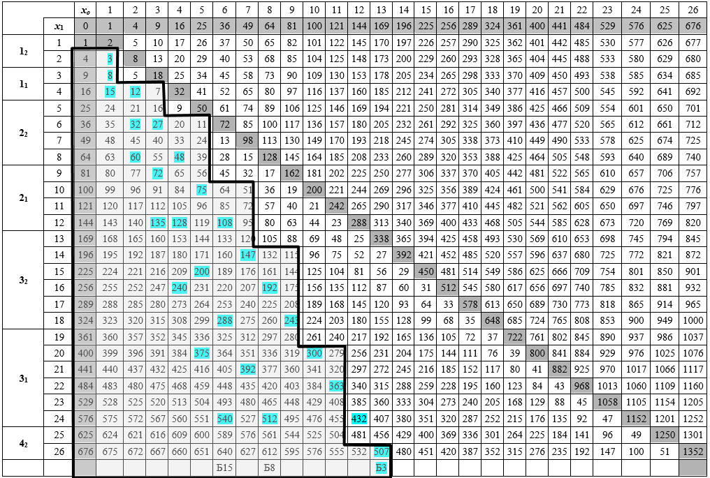
Note that the cells of such a discrete plane are unique, and the values in them can be repeated. With this definition, the parity of the values in the cells corresponds to an alternating order, like the color of the cells on a chessboard. Cells in this case will be called even or odd, respectively. The cells placed under the main diagonal form a half-plane, which we will call Г 2- (Г from the word hyperbole), and above the main diagonal - К = Г 2+ (К from the word circle). We denote the generalized model by Г s∓ , where s - can take the values 2, 3, ..., etc.
 |  |
| Equidistant hyperbole N = x 1 2 - x 0 2 | G and K - half-planes and hyperbole |
Elements of the model are cells (an analogue of a point on a plane), straight lines (sets of cell-points adjacent to one of the sides or a vertex, one to the other) horizontal (N i ) , vertical (V i ) , inclined (sets of adjacent vertex-cell cells or cells without contact, forming the direction of the lines with gaps - rays): long (D i ) and short (K i )diagonals that contain either only even values and are called even or odd diagonals formed by odd cells. Short diagonals end and begin at the points of the coordinate axes with matching coordinates (diagonal numbers). Long diagonals (D i ) run parallel to the main (with number (D 0 ) ) have only starting points on the coordinate axes and continue down to ∞. Their position above and below (D 0 ) is characterized by coincident numbers and, to distinguish them, the diagonals of the upper half-plane are equipped with an additional (+) sign (D i + ) . Odd diagonal (D1 + ) begins at the axis x 0 cell 1 and comprises in its cells of odd numbers. The odd diagonal D 1 begins on the x 1 axiswith a cell with N = 1 and contains all odd numbers, sorted in ascending order. This ensures the requirement for the NRF model to contain all odd numbers.
Within the framework of such a model, a convenient opportunity arises to study hypothetical numerical patterns and solve, for example, the problems of determining and localizing Pythagorean triples of numbers, factoring a number (factorization), determining multiple cells containing the same values, their location and other number-theoretic problems. In addition, there are good opportunities for visual display of results.
Dependencies of numbers in organized cells
Under the organization of cells we mean the belonging of some (semantically allocated) cells to a certain image, defined by the mathematical dependence of either coordinates, or values in the cells, or both. We will use the properties of the resulting images to solve number-theoretic problems, in particular, for the FBCH. We begin our consideration with very simple images of straight lines, rays. G 2- - the model provides their visualization.
Example 1 . Consider the lower half-plane Г 2- and the values of numbers in the cells with coordinates (x 1 , x 0 ) , where the coordinate x 1 is proportional to the other x 0 coordinatex 1 = kx 0 , the proportionality coefficient changes monotonously k = 2,3,4, .... ∞ , which is briefly written as k = 2 (1) ∞ . With a change in the coordinate x 0 = 0 (1) ∞ , i.e., from zero to infinity in steps of 1 and for a fixed value of k, cells and natural values in them belonging to lines (rays) with discontinuities will be calculated. So for k = 2 , the resulting cells are located in the middle of the horizontal segments of the lower half-plane, and the line takes the form of a bisector beam (marked B3 ) of the lower half-plane. For k = 3the resulting cells are located in the middle of segments of short diagonals of the lower half-plane, and the line takes the form of another beam-bisector (marked B8 ) of the lower half-plane.
Let a certain number N ∊ Г 2- be given , and it lies in one of the cells of the inclined line (ray) formed by the conditions of the example. Then we can obtain the following relation for the ray model:
for k = 2 , we have N (x 1 , x 0 ) = x 1 2 - x 0 2 = (kx 0 ) 2 - x 0 2 = x 0 2 (k 2- 1) = 3x 0 2 . Ray B3 ;
for k = 3 , we have N (x 1 , x 0 ) = x 1 2 - x 0 2 = (kx 0 ) 2 - x 0 2 = x 0 2 (k 2 - 1) = 8x 0 2 . Beam B8 ;
for k = 4 , we have N (x 1 , x 0 ) = x 1 2 - x 0 2 = (kx 0) 2 - x 0 2 = x 0 2 (k 2 - 1) = 15x 0 2 . Ray B15 ;
for k = 5 , we have N (x 1 , x 0 ) = x 1 2 - x 0 2 = (kx 0 ) 2 - x 0 2 = x 0 2 (k 2 - 1) = 24x 0 2 . Beam B24 ;
The main property of such rays for the HFBF is that the numbers in the ray cells are determined by a single coordinate x 0 , i.e. the value of N (x 1 , x 0 ) = N (kx 0 , x 0 ) = (kx 0 ) 2 - x 0 2 = x 0 2 (k 2 - 1) in a cell belonging to one of the rays becomes a function of only one x coordinate 0 . The presence of the number N, the fact that a particular beam belongs to its cell, they provide the determination of the second coordinate and the solution of the FBCH in a fraction of a second, which practically does not depend on the number of bits. The value of the second coordinate is found from the ratio of the half-plane beam model x 1 = kx 0 . It follows from the presence of both cell coordinates that all line numbers in such cells are factorized by elementary actions and almost instantly. The given simple illustrative examples convince us of this.
Indeed, N (x 1 , x 0 ) = x 1 2 - x 0 2 = (x 1 + x 0 ) (x 1 -x0 ) = p ∙ q.
Example 2 . Confirmation of the efficiency of the model by a computational experiment. Let N = 968 and N = 507 ∊ Г 2- - modelsbe given for factorization, and each one lies in one of the cells of the oblique straight line formed by the relation for some k , for example, k = 2 we get N (x 1 , x 0 ) = x 1 2 - x 0 2 = (kx 0 ) 2 - x 0 2 = x 0 2 (k 2 - 1) = 3x 0 2 = 968.
- Checks whether a given number belongs to one of the possible rays of the half-plane Г 2- . The value N = 968 is checked for belonging to beam B3 , we divide N by 3 , the number N = 968 is not completely divided by 3 , we check that it belongs to the next beam B8 , we divide by 8 . 968/8 = 121 = 11 2 = x 0 2 .
- It turned out that the number N = 968 lies in a cell belonging to beam B8 , and the cell has a coordinate x 0 = 11 . The second coordinate of the cell is determined from the ratio of the beam model x 1 = kx 0 = 3 ∙ 11 = 33 . The presence of cell coordinates provides the factorization of the number in it: N (x 1 , x 0 ) = x 1 2 - x 0 2 = (x 1 + x 0 ) (x 1- x 0 ) = (33 + 11) (33-11 ) = 44 ∙ 22 = 968 . Factoring completed successfully.
For the second number N = 507, we perform the same actions.
- The first check confirms that the B3 cell belongs to the cell with the number N = 507 , and gives the division result 507/3 = 169 = 13 2 = x 0 2 . The cell coordinate x 0 = 13 . Another coordinate is x 1 = 2x 0 = 2 ∙ 13 = 26 .
This coordinate can be found in another way. It has an independent value (value) and is applicable in other situations. From the general relation N (x 1 , x 0 ) = x 1 2 - x 0 2 = (kx 0 ) 2 - x0 2 = x 0 2 (k 2 - 1) = 3x 0 2 = 507 . - We find by dividing N / 3 = 507/3 = 169 the value x 0 2 and summing N of this square, we find the square of another coordinate x 1 2 = N + x 0 2 = 507 + 169 = 676 . From where x 1 = 26 and x 0 = 13 . Then the factorization of the number N represented by the difference of squares, N = 507 = x 1 2 - x 0 2 = (26 - 13) (26 + 13) = 13 ∙ 39 = 507 , is successfully performed and completed.
Used sources
1. Gelfond A.O., Linnik Yu.V. Elementary methods in analytic number theory. -M .: GIFFL, 1962.-272с.
2. Linnik Yu.V. On the representation of large numbers by a sum of seven cubes, Mat. Sat 12 (54), (1943), 220-224.
3. Linnik Yu.V. On the decomposition of large numbers into seven cubes, DAN 36 (1942), 179-180
4. Manin Yu.N., Panchishkin A.A. Introduction to modern number theory. –M .: ICMMO, 2013. - 552s.