Each of us perceives the texts in their own way, be it news on the Internet, poetry or classic novels. The same applies to algorithms and methods of machine learning, which, as a rule, perceive texts in mathematical form, in the form of a multidimensional vector space.

The article is devoted to the visualization of multidimensional vector representations of words using t-SNE of the calculated Word2Vec. Visualization will allow you to more fully understand how Word2Vec works and how to interpret the relationship between word vectors before using them further in neural networks and other machine learning algorithms. The article focuses on visualization, further research and data analysis are not considered. We use Google News articles and L.N.'s classic works as a data source. Tolstoy. The code will be written in Python in Jupyter Notebook.

T-distributed Stochastic Neighbor Embedding

T-SNE is a machine learning algorithm for data visualization based on the nonlinear dimension reduction method, which is described in detail in the original article [1] and on Habré . The basic t-SNE principle of operation is to reduce pairwise distances between points while maintaining their relative position. In other words, the algorithm maps multidimensional data to a space of a lower dimension, while maintaining the structure of the neighborhood of points.

Vector representations of words and Word2Vec

First of all, we need to present the words in vector form. For this task, I chose the Word2Vec distribution semantics utility, which is designed to display the semantic meaning of words in a vector space. Word2Vec finds relationships between words according to the assumption that semantically close words are found in similar contexts. More information about Word2Vec can be found in the original article [2], as well as here and here .

As input, we will take articles from Google News and novels by L.N. Tolstoy. In the first case, we will use the pre-trained on Google News (about 100 billion words) vectors, published by Google on the project page .

import gensim
model = gensim.models.KeyedVectors.load_word2vec_format('GoogleNews-vectors-negative300.bin', binary=True)

In addition to the pre-trained vectors using the Gensim library [3], we will train another model on the texts of L.N. Tolstoy. Since Word2Vec accepts an array of sentences as input, we use the pre-trained Punkt Sentence Tokenizer model from the NLTK package to automatically break the text into sentences. The model for the Russian language can be downloaded from here .

import re
import codecs
defpreprocess_text(text):
    text = re.sub('[^a-zA-Zа-яА-Я1-9]+', ' ', text)
    text = re.sub(' +', ' ', text)
    return text.strip()
defprepare_for_w2v(filename_from, filename_to, lang):
    raw_text = codecs.open(filename_from, "r", encoding='windows-1251').read()
    with open(filename_to, 'w', encoding='utf-8') as f:
        for sentence in nltk.sent_tokenize(raw_text, lang):
            print(preprocess_text(sentence.lower()), file=f)

Next, using the Gensim library, we will teach the Word2Vec-model with the following parameters:

• size = 200 is the dimension of the attribute space;
• window = 5 - the number of words from the context that the algorithm analyzes;
• min_count = 5 - the word must occur at least five times for the model to take it into account.

import multiprocessing
from gensim.models import Word2Vec
deftrain_word2vec(filename):
    data = gensim.models.word2vec.LineSentence(filename)
    return Word2Vec(data, size=200, window=5, min_count=5, workers=multiprocessing.cpu_count())

Visualizing vector representations of words with t-SNE

T-SNE is extremely useful for visualizing the similarities between objects in a multidimensional space. With the increase in the amount of data, it becomes more and more difficult to build a visual graph, therefore, in practice, similar words are combined into groups for further visualization. Take for example a few words from a dictionary of a pre-Google2 Word2Vec model.

keys = ['Paris', 'Python', 'Sunday', 'Tolstoy', 'Twitter', 'bachelor', 'delivery', 'election', 'expensive',
        'experience', 'financial', 'food', 'iOS', 'peace', 'release', 'war']
embedding_clusters = []
word_clusters = []
for word in keys:
    embeddings = []
    words = []
    for similar_word, _ in model.most_similar(word, topn=30):
        words.append(similar_word)
        embeddings.append(model[similar_word])
    embedding_clusters.append(embeddings)
    word_clusters.append(words)

Figure 1. Groups of similar words from Google News with different preplexity parameter values.

Next, go to the most remarkable fragment of the article - the configuration of t-SNE. Here, first of all, attention should be paid to the following hyperparameters:

• n_components - the number of components, i.e., the dimension of the value space;
• perplexity is perplexion, the value of which in t-SNE can be equated to the effective number of neighbors. It is related to the number of nearest neighbors, which is used in other models that study on the basis of manifolds (see picture above). Its value is recommended [1] to set in the range of 5-50;
• init is the type of initial initialization of vectors.

tsne_model_en_2d = TSNE(perplexity=15, n_components=2, init='pca', n_iter=3500, random_state=32)
embedding_clusters = np.array(embedding_clusters)
n, m, k = embedding_clusters.shape
embeddings_en_2d = np.array(tsne_model_en_2d.fit_transform(embedding_clusters.reshape(n * m, k))).reshape(n, m, 2)

Below is a script for constructing two-dimensional graphics using Matplotlib, one of the most popular libraries for visualizing data in Python.


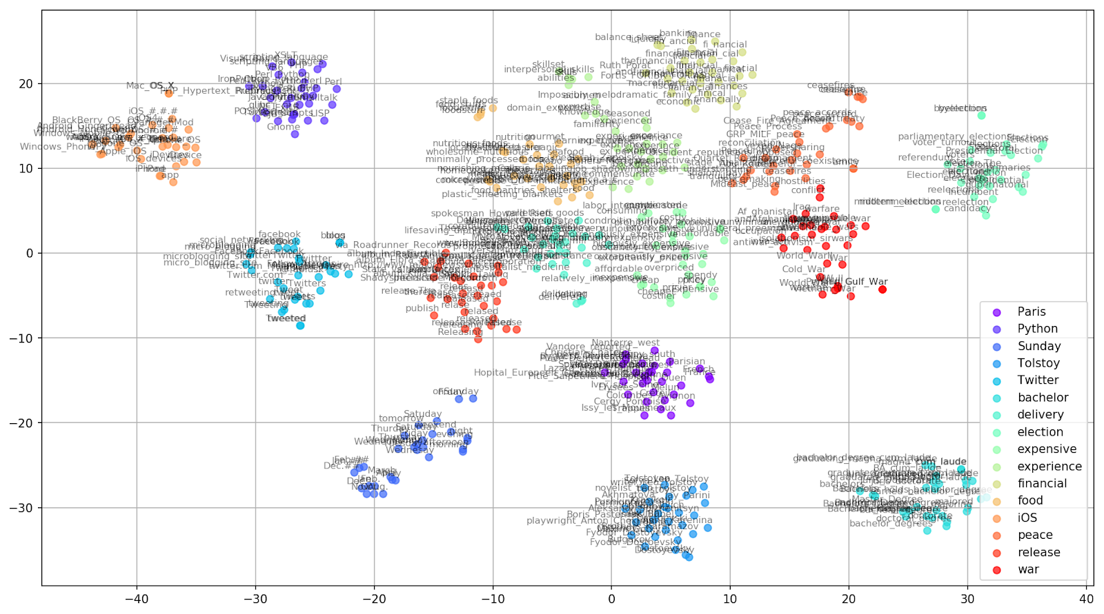
Figure 2. Groups of similar words from Google News (preplexity = 15).

from sklearn.manifold import TSNE
import matplotlib.pyplot as plt
import matplotlib.cm as cm
import numpy as np
% matplotlib inline
deftsne_plot_similar_words(labels, embedding_clusters, word_clusters, a=0.7):
    plt.figure(figsize=(16, 9))
    colors = cm.rainbow(np.linspace(0, 1, len(labels)))
    for label, embeddings, words, color in zip(labels, embedding_clusters, word_clusters, colors):
        x = embeddings[:,0]
        y = embeddings[:,1]
        plt.scatter(x, y, c=color, alpha=a, label=label)
        for i, word in enumerate(words):
            plt.annotate(word, alpha=0.5, xy=(x[i], y[i]), xytext=(5, 2), 
                         textcoords='offset points', ha='right', va='bottom', size=8)
    plt.legend(loc=4)
    plt.grid(True)
    plt.savefig("f/г.png", format='png', dpi=150, bbox_inches='tight')
    plt.show()
tsne_plot_similar_words(keys, embeddings_en_2d, word_clusters)

Sometimes it is necessary to build not separate clusters of words, but the entire vocabulary. For this purpose, let's analyze the “Anna Karenina”, the great history of passion, treason, tragedy and redemption.

prepare_for_w2v('data/Anna Karenina by Leo Tolstoy (ru).txt', 'train_anna_karenina_ru.txt', 'russian')
model_ak = train_word2vec('train_anna_karenina_ru.txt')
words = []
embeddings = []
for word in list(model_ak.wv.vocab):
    embeddings.append(model_ak.wv[word])
    words.append(word)
tsne_ak_2d = TSNE(n_components=2, init='pca', n_iter=3500, random_state=32)
embeddings_ak_2d = tsne_ak_2d.fit_transform(embeddings)

deftsne_plot_2d(label, embeddings, words=[], a=1):
    plt.figure(figsize=(16, 9))
    colors = cm.rainbow(np.linspace(0, 1, 1))
    x = embeddings[:,0]
    y = embeddings[:,1]
    plt.scatter(x, y, c=colors, alpha=a, label=label)
    for i, word in enumerate(words):
        plt.annotate(word, alpha=0.3, xy=(x[i], y[i]), xytext=(5, 2), 
                     textcoords='offset points', ha='right', va='bottom', size=10)
    plt.legend(loc=4)
    plt.grid(True)
    plt.savefig("hhh.png", format='png', dpi=150, bbox_inches='tight')
    plt.show()
tsne_plot_2d('Anna Karenina by Leo Tolstoy', embeddings_ak_2d, a=0.1)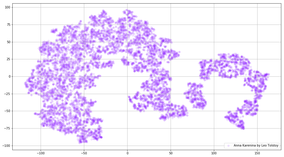

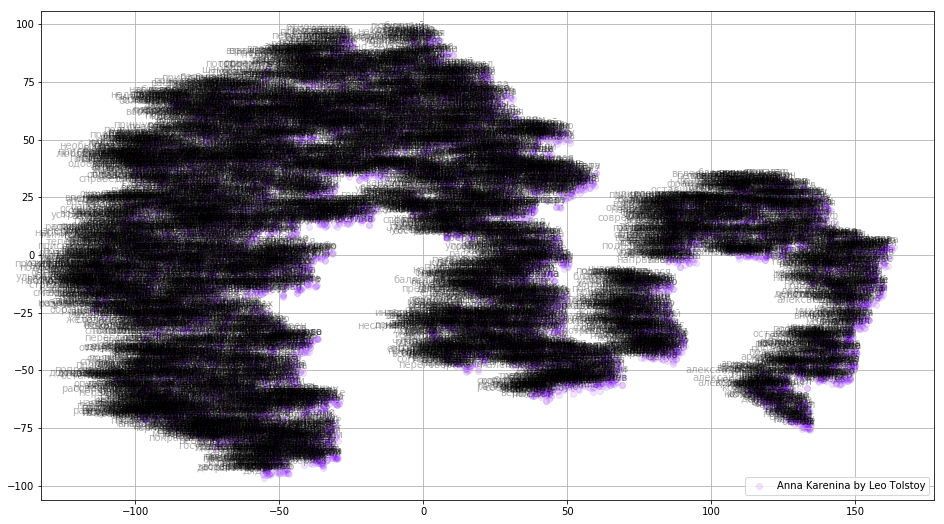
Figure 3. Visualization of the dictionary of the Word2Vec-model trained in the novel “Anna Karenina”.

The picture can become even more informative if we use three-dimensional space. Take a look at War and Peace, one of the main novels of world literature.

prepare_for_w2v('data/War and Peace by Leo Tolstoy (ru).txt', 'train_war_and_peace_ru.txt', 'russian')
model_wp = train_word2vec('train_war_and_peace_ru.txt')
words_wp = []
embeddings_wp = []
for word in list(model_wp.wv.vocab):
    embeddings_wp.append(model_wp.wv[word])
    words_wp.append(word)
tsne_wp_3d = TSNE(perplexity=30, n_components=3, init='pca', n_iter=3500, random_state=12)
embeddings_wp_3d = tsne_wp_3d.fit_transform(embeddings_wp)

from mpl_toolkits.mplot3d import Axes3D
deftsne_plot_3d(title, label, embeddings, a=1):
    fig = plt.figure()
    ax = Axes3D(fig)
    colors = cm.rainbow(np.linspace(0, 1, 1))
    plt.scatter(embeddings[:, 0], embeddings[:, 1], embeddings[:, 2], c=colors, alpha=a, label=label)
    plt.legend(loc=4)
    plt.title(title)
    plt.show()
tsne_plot_3d('Visualizing Embeddings using t-SNE', 'War and Peace', embeddings_wp_3d, a=0.1)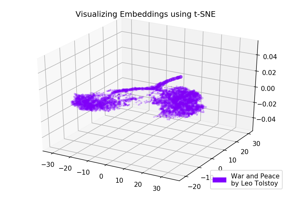

Figure 4. Visualization of the dictionary of the Word2Vec model trained in the novel War and Peace.

Sources

The code is available on github . There you can also find the code for rendering animations.

Sources

1. Maaten L., Hinton G. Visualizing data using t-SNE // Journal of machine learning learning. - 2008. - V. 9. - p. 2579-2605.
2. Representations of Words and Their Compositionality // Advances in Neural Information Processing Systems . - 2013. - p. 3111-3119.
3. Rehurek R., Sojka P. Software framework for topic modeling with large-scale corpora // In Proceedings of the LREC 2010 Workshop on NLP Frameworks. - 2010.