Bresenham's Algorithm in a Soldering Furnace - Theory

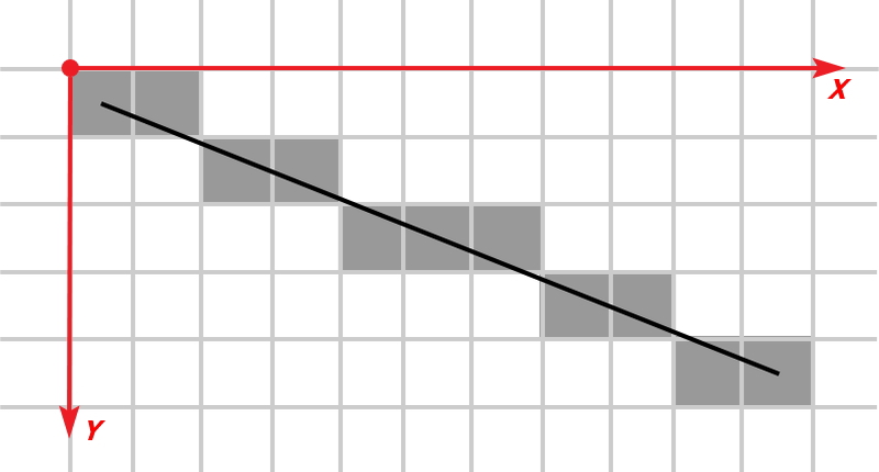The Bresenham algorithm is one of the oldest algorithms in computer graphics. It would seem, how can one apply the algorithm for constructing raster lines when creating a home soldering furnace? It turns out that you can, and with a very decent result. Looking ahead, I’ll say that this algorithm is very well fed by a low-power 8-bit microcontroller. But first things first.

The Bresenham algorithm is an algorithm that determines which points of a two-dimensional raster need to be colored to get a close approximation of a straight line between two given points. The essence of the algorithm is to determine for each column X (see the figure) which row Y is closest to the line and draw a point.

Now let's see how a similar algorithm will help us in controlling TENs in an electric furnace.

The heater is powered by a voltage of 220V / 50Hz. Take a look at the chart.


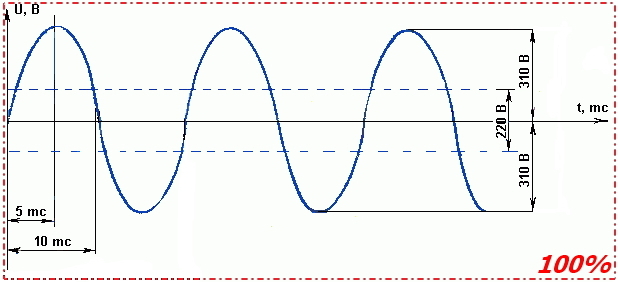
When applying such voltage in its pure form to the input of the electric heater, we will get 100% heating output. Everything is simple.


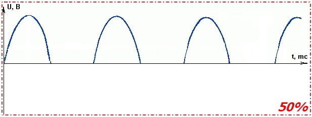
What will happen if only a positive half-wave of the mains voltage is applied to the input of the heating element? That's right, we get 50% of the heating output.


If you give every third half-wave, we get 33% power.

As an example, take a 10% gradation of the output power and a time span of 100ms, which is equivalent to 10 half-waves of the mains voltage. Draw a 10x10 grid and imagine that the Y axisthis is the axis of the output power. Draw a straight line from 0 to the required power value.



Tracing addiction?
By increasing the time period to 1 second, you can get a gradation of the output power of 1%. Get a 100x100 grid with all the consequences.

And now for the good part:
The Bresenham algorithm can be built in a loop so that at each step along the X axis, you simply track the error value, which means the vertical distance between the current y value and the exact y value for the current x . Whenever we increase x , we increase the error value by the amount of slope. If the error exceeds 0.5, the line is closer to the next y, therefore, we increase y by one (read - we skip one half-wave of voltage), while decreasing the error value by 1.

This approach can easily be reduced to cyclic integer addition (more on this later in the description of the MK operation algorithm in the next article), which is an undoubted plus for microcontrollers.

I deliberately did not load you with formulas. The algorithm is elementary, it is easy to google. I just want to show its applicability in circuitry. To control the load, a typical MOC3063 triac optocoupler wiring diagram with a zero detector will be used.



With this approach, there are a number of advantages.

• Minimal interference in the network due to frequent switching of a large load, switching on / off will occur at the moments when the voltage passes through zero.
• A very simple algorithm - all calculations come down to working with integers, which is good for a microcontroller.
• There is no need to fence zero voltage transition detector (hello MOC3063). Even if the MK simply pulls the timer, opening the optocoupler, the error will not be critical.

To be continued.