Software renderer - 1: materiel
Software rendering is the process of building an image without using a GPU. This process can go in one of two modes: in real time (the calculation of a large number of frames per second is necessary for interactive applications, for example, games) and in the "offline" mode (in which time that can be spent on calculating one frame, not limited so strictly - calculations can last hours or even days). I will only consider real-time rendering mode.
This approach has both disadvantages and advantages. The obvious drawback is the performance - the CPU is not able to compete with modern graphics cards in this area. The advantages include independence from the video card - that is why it is used as a replacement for hardware rendering in cases where the video card does not support one or another feature (the so-called software fallback). There are projects whose purpose is to completely replace hardware rendering with software, for example, WARP, which is part of Direct3D 11.
But the main advantage is the ability to write such a renderer yourself. It serves educational purposes and, in my opinion, it is the best way to understand the underlying algorithms and principles.
This is exactly what will be discussed in the series of these articles. We will start with the ability to fill the pixel in the window with the specified color and build on this the ability to draw a three-dimensional scene in real time, with moving textured models and lighting, as well as the ability to move around this scene.
But in order to display at least the first polygon, it is necessary to master the mathematics on which it is built. The first part will be devoted to it, so it will have many different matrices and other geometry.
At the end of the article there will be a link to the github of the project, which can be considered as an example of implementation.
Despite the fact that the article will describe the very basics, the reader still needs a certain foundation for its understanding. This foundation: the basics of trigonometry and geometry, understanding Cartesian coordinate systems and basic operations on vectors. Also, it’s a good idea to read some article on the basics of linear algebra for game developers (for example, this), since I will skip descriptions of some operations and dwell only on the most important, from my point of view. I will try to show why some important formulas are derived, but I will not describe them in detail - you can do the full proof yourself or find it in the relevant literature. In the course of the article, I will first try to give algebraic definitions of a particular concept, and then describe their geometric interpretation. Most of the examples will be in two-dimensional space, since my skills in drawing three-dimensional and, especially, four-dimensional spaces leave much to be desired. Nevertheless, all examples can be easily generalized to spaces of other dimensions. All articles will be more focused on the description of algorithms, rather than on their implementation in the code.
Vector is one of the key concepts in three-dimensional graphics. And although linear algebra gives it a very abstract definition, in the framework of our tasks, by an n- dimensional vector we can simply mean an array of n real numbers: an element of the space R n : The
interpretation of these numbers depends on the context. The two most common: these numbers specify the coordinates of a point in space or directional displacement. Despite the fact that their presentation is the same ( n real numbers), their concepts are different - the point describes the position in the coordinate system, and the offset does not have the position as such. In the future, we can also determine the point using the offset, implying that the offset comes from the origin.
As a rule, in most game and graphic engines there is a class of a vector precisely as a set of numbers. The meaning of these numbers depends on the context in which they are used. This class defines methods for working with geometric vectors (for example, calculating a vector product) and for points (for example, calculating the distance between two points).
In order to avoid confusion, within the framework of the article we will no longer understand the word “vector” as an abstract set of numbers, but we will call it the offset.
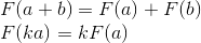
The only operation on vectors that I want to dwell on in detail (due to its fundamental nature) is a scalar product. As the name implies, the result of this work is a scalar, and it is determined by the following formula:

A scalar work has two important geometric interpretations.
This section is intended to prepare the basis for the introduction of matrices. I, using the example of global and local systems, will show for what reasons several coordinate systems are used, and not one, and how to describe one coordinate system relative to another.
Imagine that we had a need to draw a scene with two models, for example:
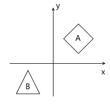
What coordinate systems naturally follow from such a statement? The first is the coordinate system of the scene itself (which is shown in the figure). This is the coordinate system that describes the world that we are going to draw - that is why it is called “world” (it will be indicated by the word “world” in the pictures). She "ties" all the objects of the scene together. For example, the coordinates of the center of object A in this coordinate system are (1, 1), and the coordinates of the center of the object B are (-1, -1) .
Thus, one coordinate system already exists. Now you need to think about in what form the models that we will use in the scene come to us.
For simplicity, we assume that the model is described simply by a list of points ("peaks") of which it consists. For example, model B consists of three points that come to us in the following format:
v 0 = (x 0 , y 0 )
v 1 = (x 1 , y 1 )
v 2 = (x 2 , y 2 )
At first glance, it would be great if they were already described in the “world” system we need! Imagine, you add a model to the scene, and it is already where we need it. For model B, it could look like this:
v 0 = (-1.5, -1.5)
v 1 = (-1.0, -0.5)
v 2 = (-0.5, -1.5)
But this approach will not work. There is an important reason for this: it makes it impossible to use the same model again in different scenes. Imagine you were given a Model B, which was modeled so that when you add it to the scene, it appears in the right place for us, as in the example above. Then, suddenly, the demand changed - we want to move it to a completely different position. It turns out that the person who created this model will have to move it on their own and then give it back to you. Of course, this is completely absurd. An even stronger argument is that in the case of interactive applications, a model can move, rotate, animate on stage - so what, an artist can do a model in all possible positions? That sounds even more stupid.
The solution to this problem is the “local” coordinate system of the model. We model the object in such a way that its center (or what can be arbitrarily taken as such) is located at the origin. Then we programmatically orient (move, rotate, etc.) the local coordinate system of the object to the desired position in the world system. Returning to the scene above, object A (unit square rotated 45 degrees clockwise) can be modeled as follows:

The model description in this case will look like this:
v 0 = (-0.5, 0.5)
v 1 = (0.5, 0.5)
v 2 = (0.5, -0.5)
v 3 = (-0.5, -0.5)
And, accordingly, the position in the scene of two coordinate systems - world and local object A :

This is one of the examples why the presence of several coordinate systems simplifies the life of developers (and artists!). There is also another reason - the transition to a different coordinate system can simplify the necessary calculations.
There is no such thing as absolute coordinates. A description of something always happens relative to some coordinate system. Including a description of another coordinate system.
We can build a kind of hierarchy of coordinate systems in the example above:
In our case, this hierarchy is very simple, but in real situations it can have a much stronger branching. For example, a local coordinate system of an object may have child systems responsible for the position of a particular part of the body.
Each child coordinate system can be described relative to the parent using the following values:
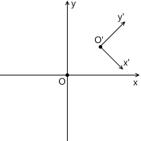
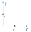
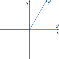
For example, in the picture below, the origin of the x'y ' system (designated as O' ) is located at the point (1, 1) , and the coordinates of its basis vectors i ' and j' are (0.7, -0.7) and (0.7, 0.7 ) respectively (which approximately corresponds to axes rotated 45 degrees clockwise).
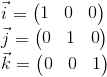
We do not need to describe the world coordinate system in relation to any other, because the world system is the root of the hierarchy, we do not care where it is located or how it is oriented. Therefore, to describe it, we use the standard basis:
The coordinates of the point P in the parent coordinate system (denoted by P parent ) can be calculated using the coordinates of this point in the child system (denoted by P child ) and the orientation of this child system relative to the parent (described using the origin of the coordinates O child and basis vectors i ' and j ' ) as follows:

Back to the example scene above. We oriented the local coordinate system of object A relative to the world:
As we already know, in the process of rendering we will need to translate the coordinates of the vertices of the object from the local coordinate system to the world. To do this, we need a description of the local coordinate system relative to the world. It looks like this: the origin at the point (1, 1) , and the coordinates of the basis vectors are (0.7, -0.7) and (0.7, 0.7) (the method of calculating the coordinates of the basis vectors after the rotation will be described later, for now, we have enough results) .
As an example, we take the first vertex v = (-0.5, 0.5) and calculate its coordinates in the world system:
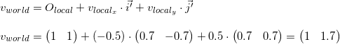
You can verify the accuracy of the result by looking at the image above.
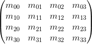
The matrix of dimension mxn is the corresponding table of numbers. If the number of columns in the matrix is equal to the number of rows, then the matrix is called square. For example, a 3 x 3 matrix is as follows:

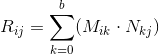
Suppose we have two matrices: M (dimension axb ) and N (dimension cxd ). The expression R = M · N is defined only if the number of columns in the matrix M is equal to the number of rows in the matrix N (i.e., b = c ). The dimension of the resulting matrix will be equal to axd (i.e., the number of rows is equal to the number of rows M and the number of columns is the number of columns in N ), and the value located at position ij is calculated as the scalar product of the i- th row M by j-th column N :
If the result of the multiplication of two matrices M · N is defined, then this does not mean at all that the multiplication in the opposite direction is also determined - N · M (the number of rows and columns may not coincide). In general, the operation of multiplication matrixes so as not commutative: M · N · M ≠ N .
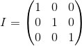
A unit matrix is a matrix that does not change another matrix multiplied by it (i.e., M · I = M ) - a kind of analogue of the unit for ordinary numbers:
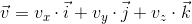
We can also represent the vector as a matrix. There are two possible ways to do this, which are called `` row vector '' and `` column vector ''. As the name implies, a row vector is a vector represented as a matrix with one row, and a column vector is a vector represented as a matrix with one column.
Row
vector : Column vector:

Next, we will very often encounter the operation of multiplying a matrix by a vector (for which it will be explained in the next section), and, looking ahead, the matrices with which we will work will have either 3 x 3 or 4 x 4 .
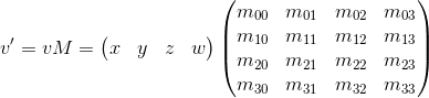
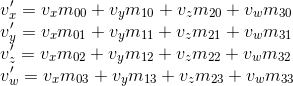
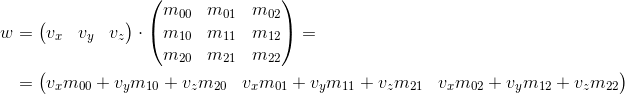
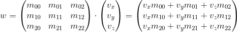
Consider how we can multiply a three-dimensional vector by a 3 x 3 matrix(similar considerations apply to other dimensions). By definition, two matrices can be multiplied if the number of columns in the first matrix is equal to the number of rows in the second. Thus, since we can represent the vector both as a 1 x 3 matrix (row vector) and as a 3 x 1 matrix (column vector), we get two possible options:
As you can see, we get a different result in each case. This can lead to random errors if the API allows you to multiply the vector by the matrix on both sides, because, as we will see later, the transformation matrix implies that the vector will be multiplied by it in one of two ways. So, in my opinion, in the API it is better to stick to only one of two options. In the framework of these articles I will use the first option - i.e. the vector is multiplied by the matrix on the left. If you decide to use a different order, then in order to get the correct results, you will need to transpose all the matrices that will be found later in this article, and replace the word “row” with “column”. It also affects the order of matrix multiplication in the presence of several transformations (more will be discussed later).
It can also be seen from the multiplication result that the matrix in a certain way (depending on the value of its elements) changes the vector that was multiplied by it. It can be such transformations as rotation, scaling, and others.
Another extremely important property of the matrix multiplication operation, which will be useful to us in the future, is distributivity with respect to addition:

As we saw in the previous section, the matrix transforms the vector multiplied by it in a certain way.
Once again we recall that any vector can be represented as a linear combination of basis vectors:

Multiply this expression by a matrix:

Using distributiveness with respect to addition, we get:

We already saw this before when we considered how to transfer the coordinates of a point from a child system to a parent system, then this it looked like this (for three-dimensional space):

There are two differences between the two expressions - there is no movement in the first expression ( O child , we will examine this point later in more detail when we talk about whether neural and affine transformations), and the vectors i ' , j'and k ' are replaced by iM , jM and kM respectively. Consequently, iM , jM and kM - is affiliated basis vectors of the coordinate system and we translate point v child (v x , v y , v y ) of the coordinate system of this child to the parent ( v transformed = v parent M ).
The transformation process can be represented as follows by the example of counterclockwise rotation ( xy is the original, parent coordinate system, x'y '- daughter, obtained as a result of transformation):
Just in case, to make sure that we understand the meaning of each of the vectors used above, we list them again:
Now consider what happens when the basis vectors are multiplied by the matrix M :

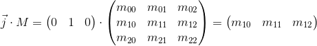
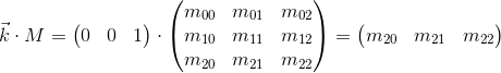
It can be seen that the basis vectors of the new daughter coordinate system obtained by multiplying by the matrix M coincide with the rows of the matrix. This is the very geometric interpretation that we were looking for. Now, having seen the transformation matrix, we will know where to look in order to understand what it is doing - just imagine its rows as the basis vectors of the new coordinate system. The transformation taking place with the coordinate system will be the same as the transformation taking place with the vector multiplied by this matrix.
We can also combine the transformations represented in the form of matrices by multiplying them by each other:

Thus, matrices are a very convenient tool for describing and combining transformations.
First, consider the most commonly used linear transformations. A linear transformation is a transformation that satisfies two properties:
An important consequence is that a linear transformation cannot contain movement (this is also the reason why the O child term was absent in the previous section), because, according to the second formula, 0 always maps to 0 .
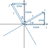
Consider rotation in two-dimensional space. This is a transformation that rotates the coordinate system by a given angle. As we already know, it is enough for us to calculate the new coordinate axes (obtained after rotation by a given angle), and use them as rows of the transformation matrix. The result is easily obtained from the basic geometry:

Example:

The result for rotation in three-dimensional space is obtained in a similar way, with the only difference being that we rotate a plane composed of two coordinate axes, and fix the third (around which the rotation occurs). For example, the rotation matrix around the x axis is as follows:

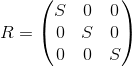
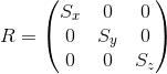
We can change the scale of the object relative to all axes by applying the following matrix: The
axes of the transformed coordinate system will be directed in the same way as the original coordinate system, but will require S times longer for one unit of measurement:
Example:
Scaling with the same coefficient relative to all axes called uniform. But we can also scale with different coefficients along different axes (nonuniform):
As the name implies, this transformation produces a shift along the coordinate axis, leaving the remaining axes intact:
Accordingly, the shift matrix of the y axis looks as follows:

Example:

The matrix for three-dimensional space is constructed in a similar way. For example, an option for shifting the x axis :

Although this transformation is used very rarely, it will come in handy in the future when we consider affine transformations.
We already have a decent number of transformations in our stock, which can be represented as a 3 x 3 matrix, but we lack one more thing - moving. Unfortunately, expressing movement in three-dimensional space with 3 x 3matrices are impossible, since displacement is not a linear transformation. The solution to this problem is homogeneous coordinates, which we will consider later.
Our final goal is to depict a three-dimensional scene on a two-dimensional screen. Thus, we must in one way or another design our scene on a plane. There are two most commonly used types of projections - orthographic and central (another name - perspective).
When the human eye looks at a three-dimensional scene, objects farther away from it become smaller in the final image that a person sees - this effect is called perspective. Orthographic projection ignores the perspective, which is a useful property when working in various CAD systems (as well as in 2D games). The central projection has this property and therefore adds a significant share of realism. In this article we will consider only her.
Unlike orthographic projection, the lines in the perspective projection are not parallel to each other, but intersect at a point called the center of the projection. The projection center is the “eye” with which we look at the scene - a virtual camera:
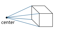
The image is formed on a plane located at a given distance from the virtual camera. Accordingly, the greater the distance from the camera, the larger the projection size:

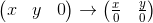
Consider the simplest example: the camera is located at the origin, and the projection plane is at a distance d from the camera. We know the coordinates of the point we want to project: (x, y, z) . Find the coordinate x p of the projection of this point on the plane:
Two similar triangles are visible in this picture - CDP and CBA (at three angles):
Respectively, relations between the sides are preserved:
We get the result for x- coordinates:

And, similarly, for y- coordinates:

Later, we will need to use this transformation to form projected image. And here the problem arises - we cannot imagine the division into z- coordinates in three-dimensional space using a matrix. The solution to this problem, as in the case of the displacement matrix, are homogeneous coordinates.
To date, we have encountered two problems:
Both of these problems are solved using uniform coordinates. Homogeneous coordinates - a concept from projective geometry. Projective geometry studies projective spaces, and to understand the geometric interpretation of homogeneous coordinates, you need to get to know them.
Below we will consider definitions for two-dimensional projective spaces, since they are easier to depict. Similar considerations apply to three-dimensional projective spaces (we will use them in the future).
We define a ray in the space R 3 as follows: a ray is a set of vectors of the form kv ( k is a scalar, v is a nonzero vector, an element of the space R 3) Those. the vector v defines the direction of the ray:

Now we can move on to the definition of projective space. The projective plane (i.e., the projective space with a dimension equal to two) P 2 associated with the space R 3 is the set of rays in R 3 . Thus, a “point” in P 2 is a ray in R 3 .
Accordingly, two vectors in R 3 define the same element in P 2 , if one of them can be obtained by multiplying the second by some scalar (since in this case they lie on the same ray):

For example, the vectors (1, 1, 1) and (5, 5, 5) represent the same ray, which means they are the same “point” in the projective plane.
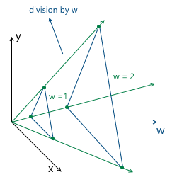
Thus, we came to uniform coordinates. Each element in the projective plane is defined by a ray of three coordinates (x, y, w) (the last coordinate is called w instead of z - the generally accepted agreement) - these coordinates are called homogeneous and determined up to a scalar. This means that we can multiply (or divide) by a scalar homogeneous coordinates, and they will still represent the same “point” in the projective plane.
In the future, we will use homogeneous coordinates to represent the affine (containing movement) transformations and projections. But before that one more question needs to be solved: how to present the model vertices given to us in the form of homogeneous coordinates? Since the "addition" to homogeneous coordinates occurs due to the addition of the third coordinate w , the question boils down to what value of w we need to use. The answer to this question is any non-zero. The difference in using different values of w lies in the convenience of working with them.
And, as will be further understood (and which is partially intuitively clear), the most convenient value of w is unity. The advantages of this choice are as follows:
Thus, we choose the value w = 1 , which means that our input data in homogeneous coordinates will now look like this (of course, the unit will already be added by us, and will not be in the model description itself):
v 0 = (x 0 , y 0 , 1)
v 1 = (x 1 , y 1 , 1)
v 2 = (x 2 , y 2 , 1)
Now we need to consider the special case when working with the w- coordinate. Namely, its equality to zero. We said above that we can choose any value of w, not equal to zero, to expand to homogeneous coordinates. We cannot take w = 0 , in particular, because it will not allow us to move this point (since, as we will see later, the movement occurs precisely due to the value in the w coordinate). Also, if the point w has zero coordinate , we can consider it as a point “at infinity”, because when we try to return to the plane w = 1, we get division by zero:
And, although we cannot use a null value for the vertices of the model, we can use it for vectors! This will lead to the fact that the vector will not be subject to displacements during transformations - which makes sense, because the vector does not describe the position. For example, when transforming a normal, we cannot move it, otherwise we will get the wrong result. We will consider this in more detail when it becomes necessary to transform vectors.
In this regard, it is often written that for w = 1 we describe a point, and for w = 0 - a vector.
As I already wrote, we used an example of two-dimensional projective projective spaces, but in reality we will use three-dimensional projective spaces, which means that each point will be described by 4 coordinates: (x, y, z, w).
Now we have all the necessary tools for describing the affinity transformations. Athenian transformations - linear transformations with subsequent displacement. They can be described as follows:

We can also use 4 x 4 matrices to describe affine transformations using homogeneous coordinates:
Consider the result of multiplying a vector represented as homogeneous coordinates and multiplying by a 4 x 4 matrix:
As you can see, the difference from transformation represented in the form of a 3 x 3 matrix consists of the 4th coordinate, as well as new terms in each of the coordinates of the form v w · m 3i . Using this, and implying w = 1, we can represent the displacement as follows:
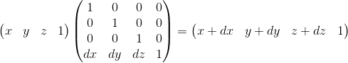
Here we can verify the correct choice of w = 1 . To represent the displacement dx, we use a term of the form w · dx / w . Accordingly, the last row of the matrix looks like (dx / w, dy / w, dz / w, 1) . In the case w = 1, we can simply omit the denominator.
This matrix also has a geometric interpretation. Recall the shift matrix, which we considered earlier. It has exactly the same format, the only difference is that the fourth axis is shifted, thus shifting the three-dimensional subspace located in the hyperplane w = 1 by the corresponding values.
A virtual camera is the “eye” with which we look at the scene. Before moving on, you need to understand how you can describe the position of the camera in space, and what parameters are necessary to form the final image.
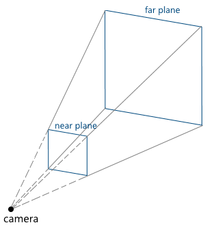
Camera parameters specify a truncated pyramid of view (view frustum), which determines which part of the scene will fall into the final image:
Consider them in turn:
We can move and rotate the camera, changing the position and orientation of its coordinate system. Code example:
Now we have all the necessary foundation in order to describe in steps the steps that are necessary to obtain an image of a three-dimensional scene on a computer screen. For simplicity, we assume that the pipeline draws one object at a time.
Inbound pipeline parameters:
At this stage, we transform the vertices of the object from the local coordinate system to the world.
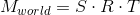
Assume that the orientation of the object in the world coordinate system is defined by the following parameters:
We call the matrices of these transformations T , R, and S, respectively. To obtain the final matrix, which will transform the object into a world coordinate system, it is enough for us to multiply them. It is important to note here that the order of matrix multiplication plays a role - this directly follows from the fact that matrix multiplication is non-commutative.
Recall that scaling occurs relative to the origin. If we first move the object to the desired point, and then apply the scale to it, we will get the wrong result - the position of the object will change again after scaling. A simple example:
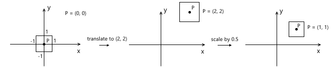
A similar rule applies to rotation - it occurs relative to the origin, which means the position of the object will change if we first move.
Thus, the correct sequence in our case is as follows: scaling - rotation - displacement:
The transition to the camera coordinate system, in particular, is used to simplify further calculations. In this coordinate system, the camera is located at the origin, and its axes are the vectors forward , right , up , which we examined in the previous section.
The transition to the camera coordinate system consists of two steps:
The first step can easily be represented as a displacement matrix by (-pos x , -pos y , -pos z ) , where pos is the position of the camera in the world coordinate system:

To implement the second point, we use the scalar product property, which we considered at the very beginning - the scalar product calculates the projection length along a given axis. Thus, in order to translate point A into the coordinate system of the camera (taking into account the fact that the camera is at the origin - we did this in the first paragraph), we just need to take its scalar product with vectors right , up , forward. We denote the point in the world coordinate system v , and the same point translated into the camera coordinate system, v ' , then:
This operation can be represented as a matrix:
Combining these two transformations, we get the transition matrix to the camera coordinate system:

Schematically, this process can be represented as follows:

As a result of the previous paragraph, we got the coordinates of the vertices of the object in the camera coordinate system. The next thing to do is to project these vertices onto a plane and “cut off” the extra vertices. The top of the object is cut off if it lies outside the viewing pyramid (i.e., its projection does not lie on the part of the plane that the viewing pyramid covers). For example, vertex v 1 in the figure below:

Both of these tasks are partially solved by the projection matrix. “Partially” - because it does not produce the projection itself, but prepares w- The vertex coordinate for this. Because of this, the name "projection matrix" does not sound very suitable (although this is a fairly common term), and I will hereinafter call it the clip matrix, since it also maps the truncated viewing pyramid to a homogeneous clipping space (homogeneous clip space).
But first things first. So, the first is preparation for projection. To do this, we put the z- coordinate of the vertex in its w- coordinate. The projection itself (i.e. division by z ) will occur with further normalization of the w-coordinate - i.e. when returning to the space w = 1 .
The next thing this matrix should do is translate the coordinates of the vertices of the object from the camera space into a homogeneous clip space. This is a space in which the coordinates of the non-truncated vertices are such that after applying the projection (i.e., dividing by the w- coordinate, since we saved the old z- coordinate in it), the coordinates of the vertex are normalized, i.e. satisfy the following conditions:

Inequality for z- coordinates may vary for different APIs. For example, in OpenGL it corresponds to what is higher. In Direct3D, the z- coordinate is displayed in the interval [0, 1] . We will use the interval accepted in OpenGL, i.e. [-1, 1] .
Such coordinates are called normalized device coordinates (or simply NDC).
Since we obtain NDC coordinates by dividing the coordinates by w , the vertices in the clipping space satisfy the following conditions:

Thus, by translating the vertices into this space, we can find out whether it is necessary to cut off the vertex by simply checking its coordinates for the inequalities above. Any vertex that does not satisfy these conditions must be cut off. Clipping itself is a topic for a separate article, since its correct implementation leads to the creation of new vertices. So far, as a quick fix, we will not draw a face if at least one of its vertices is cut off. Of course, the result is not very accurate. For example, for a machine model, it looks like this:
Total, this stage consists of the following steps:
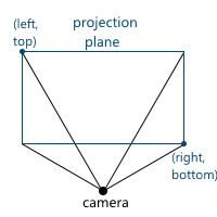
Now we will consider how we display the coordinates from the camera space to the clipping space. Recall that we decided to use the projection plane z = 1 . First we need to find a function that displays the coordinates that lie at the intersection of the pyramid of view and the projection plane in the interval [-1, 1] . To do this, find the coordinates of the points that define this part of the plane. These two points have coordinates (left, top) and (right, bottom) . We will consider only the case when the pyramid of view is symmetric with respect to the direction of the camera.
We can calculate them using viewing angles:
We

get : Similarly for top and bottom :
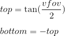
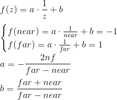
Thus, we need to map the interval [left, right] , [bottom, top] , [near, far] to [-1; 1] . We find a linear function that gives such a result for left and right :

Similarly, we get a function for bottom and top :
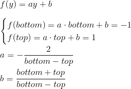
The expression for z is found differently. Instead of considering a function of the form az + b, we will consider a function a · 1 / z + b, because in the future, when we implement the depth buffer, we will need to linearly interpolate the inverse of the z-coordinate. We will not consider this issue now, and just take it for granted. We
get : Thus, we can write that the normalized coordinates are obtained as follows from the coordinates in the camera space:
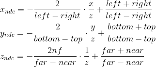
We cannot immediately apply these formulas, because division by z will occur later, when the w coordinate is normalized . We can take advantage of this, and instead calculate the following values (multiplying by z), which, after dividing by w , will result in normalized coordinates:
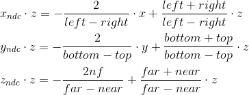
It is with these formulas that we are transforming into a cutoff space. We can write this transformation in matrix form (additionally remembering that we put z in the w- coordinate ):

To the current stage, we have the coordinates of the vertices of the object in NDC. We need to translate them into the screen coordinate system. Recall that the upper left corner of the projection plane was mapped to (-1, 1), and the lower right corner to (1, -1). For the screen, I will use the upper left corner as the origin of the coordinate system, with the axes pointing to the right and down:

This viewport transformation can be done using simple formulas:
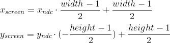
Or, in matrix form:
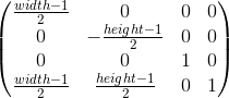
We will leave the use of z ndc until the depth buffer is implemented.
As a result, we have the coordinates of the vertices on the screen, which we use to draw.
The following is an example code that implements the pipeline using the method described above and performs rendering in wireframe mode (i.e., simply connecting the vertices with lines). It also implies that the object is described by a set of vertices and a set of indices of the vertices (faces) that its polygons consist of:
In this section, I will briefly describe how SDL2 can be used to implement rendering.
The first is, of course, initializing the library and creating the window. If only graphics are needed from the SDL, then you can initialize with the SDL_INIT_VIDEO flag :
Then, create a texture into which we will draw. I will use the ARGB8888 format , which means that 4 bytes will be allocated for each pixel in the texture - three bytes for RGB channels, and one for alpha channel.
We must not forget to “clear” the SDL and all the variables taken from it when the application exits:
We can use SDL_UpdateTexture to update the texture, which we then display on the screen. This function accepts, among others, the following parameters:
It is logical to separate the drawing functionality into a texture represented by an array of bytes into a separate class. It will allocate memory for the array, clear the texture, draw pixels and lines. Drawing a pixel can be done as follows (byte order varies depending on SDL_BYTEORDER ):
Line drawing can be implemented, for example, according to the Bresenham algorithm .
After using SDL_UpdateTexture , you need to copy the texture to SDL_Renderer and display it using SDL_RenderPresent . Together:
That's all. Link to the project: https://github.com/loreglean/lantern .
This approach has both disadvantages and advantages. The obvious drawback is the performance - the CPU is not able to compete with modern graphics cards in this area. The advantages include independence from the video card - that is why it is used as a replacement for hardware rendering in cases where the video card does not support one or another feature (the so-called software fallback). There are projects whose purpose is to completely replace hardware rendering with software, for example, WARP, which is part of Direct3D 11.
But the main advantage is the ability to write such a renderer yourself. It serves educational purposes and, in my opinion, it is the best way to understand the underlying algorithms and principles.
This is exactly what will be discussed in the series of these articles. We will start with the ability to fill the pixel in the window with the specified color and build on this the ability to draw a three-dimensional scene in real time, with moving textured models and lighting, as well as the ability to move around this scene.
But in order to display at least the first polygon, it is necessary to master the mathematics on which it is built. The first part will be devoted to it, so it will have many different matrices and other geometry.
At the end of the article there will be a link to the github of the project, which can be considered as an example of implementation.
Despite the fact that the article will describe the very basics, the reader still needs a certain foundation for its understanding. This foundation: the basics of trigonometry and geometry, understanding Cartesian coordinate systems and basic operations on vectors. Also, it’s a good idea to read some article on the basics of linear algebra for game developers (for example, this), since I will skip descriptions of some operations and dwell only on the most important, from my point of view. I will try to show why some important formulas are derived, but I will not describe them in detail - you can do the full proof yourself or find it in the relevant literature. In the course of the article, I will first try to give algebraic definitions of a particular concept, and then describe their geometric interpretation. Most of the examples will be in two-dimensional space, since my skills in drawing three-dimensional and, especially, four-dimensional spaces leave much to be desired. Nevertheless, all examples can be easily generalized to spaces of other dimensions. All articles will be more focused on the description of algorithms, rather than on their implementation in the code.
Vectors
Vector is one of the key concepts in three-dimensional graphics. And although linear algebra gives it a very abstract definition, in the framework of our tasks, by an n- dimensional vector we can simply mean an array of n real numbers: an element of the space R n : The
interpretation of these numbers depends on the context. The two most common: these numbers specify the coordinates of a point in space or directional displacement. Despite the fact that their presentation is the same ( n real numbers), their concepts are different - the point describes the position in the coordinate system, and the offset does not have the position as such. In the future, we can also determine the point using the offset, implying that the offset comes from the origin.
As a rule, in most game and graphic engines there is a class of a vector precisely as a set of numbers. The meaning of these numbers depends on the context in which they are used. This class defines methods for working with geometric vectors (for example, calculating a vector product) and for points (for example, calculating the distance between two points).
In order to avoid confusion, within the framework of the article we will no longer understand the word “vector” as an abstract set of numbers, but we will call it the offset.
Scalar product
The only operation on vectors that I want to dwell on in detail (due to its fundamental nature) is a scalar product. As the name implies, the result of this work is a scalar, and it is determined by the following formula:
A scalar work has two important geometric interpretations.
- Measuring the angle between vectors.
Consider the following triangle obtained from three vectors:
Having written the cosine theorem for it and reduced the expression, we arrive at the following record:
Since the length of a nonzero vector is by definition greater than 0, the cosine of the angle determines the sign of the scalar product and its equality to zero. We get (assuming that the angle is from 0 to 360 degrees):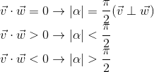
- The scalar product calculates the length of the projection of a vector onto a vector.
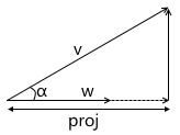
From the definition of the cosine of the angle we get: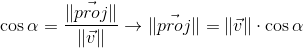
We also already know from the previous paragraph that:
Expressing the cosine of the angle from the second expression, substituting it in the first and multiplying by || w || , we get the result: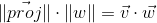
Thus, the scalar product of two vectors is equal to the projection length of the vector v onto the vector w multiplied by the length of the vector w . A frequent special case of this formula - w has a unit length and, therefore, the scalar product calculates the exact length of the projection.
This interpretation is very important because it shows that the scalar product calculates the coordinates of the point (given by the vector v , implying an offset from the origin) along the given axis. The simplest example:
We will use this in the future when constructing a transformation into a camera coordinate system.
Coordinate systems
This section is intended to prepare the basis for the introduction of matrices. I, using the example of global and local systems, will show for what reasons several coordinate systems are used, and not one, and how to describe one coordinate system relative to another.
Imagine that we had a need to draw a scene with two models, for example:
What coordinate systems naturally follow from such a statement? The first is the coordinate system of the scene itself (which is shown in the figure). This is the coordinate system that describes the world that we are going to draw - that is why it is called “world” (it will be indicated by the word “world” in the pictures). She "ties" all the objects of the scene together. For example, the coordinates of the center of object A in this coordinate system are (1, 1), and the coordinates of the center of the object B are (-1, -1) .
Thus, one coordinate system already exists. Now you need to think about in what form the models that we will use in the scene come to us.
For simplicity, we assume that the model is described simply by a list of points ("peaks") of which it consists. For example, model B consists of three points that come to us in the following format:
v 0 = (x 0 , y 0 )
v 1 = (x 1 , y 1 )
v 2 = (x 2 , y 2 )
At first glance, it would be great if they were already described in the “world” system we need! Imagine, you add a model to the scene, and it is already where we need it. For model B, it could look like this:
v 0 = (-1.5, -1.5)
v 1 = (-1.0, -0.5)
v 2 = (-0.5, -1.5)
But this approach will not work. There is an important reason for this: it makes it impossible to use the same model again in different scenes. Imagine you were given a Model B, which was modeled so that when you add it to the scene, it appears in the right place for us, as in the example above. Then, suddenly, the demand changed - we want to move it to a completely different position. It turns out that the person who created this model will have to move it on their own and then give it back to you. Of course, this is completely absurd. An even stronger argument is that in the case of interactive applications, a model can move, rotate, animate on stage - so what, an artist can do a model in all possible positions? That sounds even more stupid.
The solution to this problem is the “local” coordinate system of the model. We model the object in such a way that its center (or what can be arbitrarily taken as such) is located at the origin. Then we programmatically orient (move, rotate, etc.) the local coordinate system of the object to the desired position in the world system. Returning to the scene above, object A (unit square rotated 45 degrees clockwise) can be modeled as follows:
The model description in this case will look like this:
v 0 = (-0.5, 0.5)
v 1 = (0.5, 0.5)
v 2 = (0.5, -0.5)
v 3 = (-0.5, -0.5)
And, accordingly, the position in the scene of two coordinate systems - world and local object A :
This is one of the examples why the presence of several coordinate systems simplifies the life of developers (and artists!). There is also another reason - the transition to a different coordinate system can simplify the necessary calculations.
Description of one coordinate system relative to another
There is no such thing as absolute coordinates. A description of something always happens relative to some coordinate system. Including a description of another coordinate system.
We can build a kind of hierarchy of coordinate systems in the example above:
- world space
   - local space (object A)
   - local space (object B)
In our case, this hierarchy is very simple, but in real situations it can have a much stronger branching. For example, a local coordinate system of an object may have child systems responsible for the position of a particular part of the body.
Each child coordinate system can be described relative to the parent using the following values:
- origin point of the child system relative to the parent
- coordinates of the base vectors of the child system relative to the parent
For example, in the picture below, the origin of the x'y ' system (designated as O' ) is located at the point (1, 1) , and the coordinates of its basis vectors i ' and j' are (0.7, -0.7) and (0.7, 0.7 ) respectively (which approximately corresponds to axes rotated 45 degrees clockwise).
We do not need to describe the world coordinate system in relation to any other, because the world system is the root of the hierarchy, we do not care where it is located or how it is oriented. Therefore, to describe it, we use the standard basis:
Translation of coordinates of points from one system to another
The coordinates of the point P in the parent coordinate system (denoted by P parent ) can be calculated using the coordinates of this point in the child system (denoted by P child ) and the orientation of this child system relative to the parent (described using the origin of the coordinates O child and basis vectors i ' and j ' ) as follows:
Back to the example scene above. We oriented the local coordinate system of object A relative to the world:
As we already know, in the process of rendering we will need to translate the coordinates of the vertices of the object from the local coordinate system to the world. To do this, we need a description of the local coordinate system relative to the world. It looks like this: the origin at the point (1, 1) , and the coordinates of the basis vectors are (0.7, -0.7) and (0.7, 0.7) (the method of calculating the coordinates of the basis vectors after the rotation will be described later, for now, we have enough results) .
As an example, we take the first vertex v = (-0.5, 0.5) and calculate its coordinates in the world system:
You can verify the accuracy of the result by looking at the image above.
Matrices
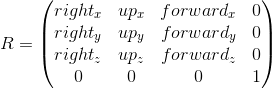
The matrix of dimension mxn is the corresponding table of numbers. If the number of columns in the matrix is equal to the number of rows, then the matrix is called square. For example, a 3 x 3 matrix is as follows:
Matrix Multiplication
Suppose we have two matrices: M (dimension axb ) and N (dimension cxd ). The expression R = M · N is defined only if the number of columns in the matrix M is equal to the number of rows in the matrix N (i.e., b = c ). The dimension of the resulting matrix will be equal to axd (i.e., the number of rows is equal to the number of rows M and the number of columns is the number of columns in N ), and the value located at position ij is calculated as the scalar product of the i- th row M by j-th column N :
If the result of the multiplication of two matrices M · N is defined, then this does not mean at all that the multiplication in the opposite direction is also determined - N · M (the number of rows and columns may not coincide). In general, the operation of multiplication matrixes so as not commutative: M · N · M ≠ N .
A unit matrix is a matrix that does not change another matrix multiplied by it (i.e., M · I = M ) - a kind of analogue of the unit for ordinary numbers:
Matrix vectors
We can also represent the vector as a matrix. There are two possible ways to do this, which are called `` row vector '' and `` column vector ''. As the name implies, a row vector is a vector represented as a matrix with one row, and a column vector is a vector represented as a matrix with one column.
Row
vector : Column vector:
Next, we will very often encounter the operation of multiplying a matrix by a vector (for which it will be explained in the next section), and, looking ahead, the matrices with which we will work will have either 3 x 3 or 4 x 4 .
Consider how we can multiply a three-dimensional vector by a 3 x 3 matrix(similar considerations apply to other dimensions). By definition, two matrices can be multiplied if the number of columns in the first matrix is equal to the number of rows in the second. Thus, since we can represent the vector both as a 1 x 3 matrix (row vector) and as a 3 x 1 matrix (column vector), we get two possible options:
- Multiplication of the vector by the matrix "left":
- Multiplication of the vector by the matrix "right":
As you can see, we get a different result in each case. This can lead to random errors if the API allows you to multiply the vector by the matrix on both sides, because, as we will see later, the transformation matrix implies that the vector will be multiplied by it in one of two ways. So, in my opinion, in the API it is better to stick to only one of two options. In the framework of these articles I will use the first option - i.e. the vector is multiplied by the matrix on the left. If you decide to use a different order, then in order to get the correct results, you will need to transpose all the matrices that will be found later in this article, and replace the word “row” with “column”. It also affects the order of matrix multiplication in the presence of several transformations (more will be discussed later).
It can also be seen from the multiplication result that the matrix in a certain way (depending on the value of its elements) changes the vector that was multiplied by it. It can be such transformations as rotation, scaling, and others.
Another extremely important property of the matrix multiplication operation, which will be useful to us in the future, is distributivity with respect to addition:
Geometric interpretation
As we saw in the previous section, the matrix transforms the vector multiplied by it in a certain way.
Once again we recall that any vector can be represented as a linear combination of basis vectors:
Multiply this expression by a matrix:
Using distributiveness with respect to addition, we get:
We already saw this before when we considered how to transfer the coordinates of a point from a child system to a parent system, then this it looked like this (for three-dimensional space):
There are two differences between the two expressions - there is no movement in the first expression ( O child , we will examine this point later in more detail when we talk about whether neural and affine transformations), and the vectors i ' , j'and k ' are replaced by iM , jM and kM respectively. Consequently, iM , jM and kM - is affiliated basis vectors of the coordinate system and we translate point v child (v x , v y , v y ) of the coordinate system of this child to the parent ( v transformed = v parent M ).
The transformation process can be represented as follows by the example of counterclockwise rotation ( xy is the original, parent coordinate system, x'y '- daughter, obtained as a result of transformation):
Just in case, to make sure that we understand the meaning of each of the vectors used above, we list them again:
- v parent - vector, which we initially multiplied by the matrix M . Its coordinates are described relative to the parent coordinate system.
- v child is a vector whose coordinates are equal to the vector v parent , but they are described relative to the child coordinate system. This is the vector v parent transformed in the same way as the base vectors (since we use the same coordinates)
- vtransformed — тот же самый вектор, что и vchild но с координатами пересчитанными относительно родительской системы координат. Это итоговый результат трансформации вектора vparent
Now consider what happens when the basis vectors are multiplied by the matrix M :
It can be seen that the basis vectors of the new daughter coordinate system obtained by multiplying by the matrix M coincide with the rows of the matrix. This is the very geometric interpretation that we were looking for. Now, having seen the transformation matrix, we will know where to look in order to understand what it is doing - just imagine its rows as the basis vectors of the new coordinate system. The transformation taking place with the coordinate system will be the same as the transformation taking place with the vector multiplied by this matrix.
We can also combine the transformations represented in the form of matrices by multiplying them by each other:
Thus, matrices are a very convenient tool for describing and combining transformations.
Linear transformations
First, consider the most commonly used linear transformations. A linear transformation is a transformation that satisfies two properties:
An important consequence is that a linear transformation cannot contain movement (this is also the reason why the O child term was absent in the previous section), because, according to the second formula, 0 always maps to 0 .
Rotation
Consider rotation in two-dimensional space. This is a transformation that rotates the coordinate system by a given angle. As we already know, it is enough for us to calculate the new coordinate axes (obtained after rotation by a given angle), and use them as rows of the transformation matrix. The result is easily obtained from the basic geometry:
Example:
The result for rotation in three-dimensional space is obtained in a similar way, with the only difference being that we rotate a plane composed of two coordinate axes, and fix the third (around which the rotation occurs). For example, the rotation matrix around the x axis is as follows:
Scaling
We can change the scale of the object relative to all axes by applying the following matrix: The
axes of the transformed coordinate system will be directed in the same way as the original coordinate system, but will require S times longer for one unit of measurement:
Example:
Scaling with the same coefficient relative to all axes called uniform. But we can also scale with different coefficients along different axes (nonuniform):
Shift
As the name implies, this transformation produces a shift along the coordinate axis, leaving the remaining axes intact:
Accordingly, the shift matrix of the y axis looks as follows:
Example:
The matrix for three-dimensional space is constructed in a similar way. For example, an option for shifting the x axis :
Although this transformation is used very rarely, it will come in handy in the future when we consider affine transformations.
We already have a decent number of transformations in our stock, which can be represented as a 3 x 3 matrix, but we lack one more thing - moving. Unfortunately, expressing movement in three-dimensional space with 3 x 3matrices are impossible, since displacement is not a linear transformation. The solution to this problem is homogeneous coordinates, which we will consider later.
Central projection
Our final goal is to depict a three-dimensional scene on a two-dimensional screen. Thus, we must in one way or another design our scene on a plane. There are two most commonly used types of projections - orthographic and central (another name - perspective).
When the human eye looks at a three-dimensional scene, objects farther away from it become smaller in the final image that a person sees - this effect is called perspective. Orthographic projection ignores the perspective, which is a useful property when working in various CAD systems (as well as in 2D games). The central projection has this property and therefore adds a significant share of realism. In this article we will consider only her.
Unlike orthographic projection, the lines in the perspective projection are not parallel to each other, but intersect at a point called the center of the projection. The projection center is the “eye” with which we look at the scene - a virtual camera:
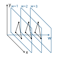
The image is formed on a plane located at a given distance from the virtual camera. Accordingly, the greater the distance from the camera, the larger the projection size:
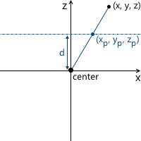
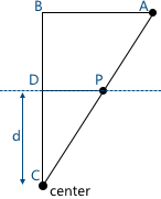
Consider the simplest example: the camera is located at the origin, and the projection plane is at a distance d from the camera. We know the coordinates of the point we want to project: (x, y, z) . Find the coordinate x p of the projection of this point on the plane:
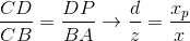
Two similar triangles are visible in this picture - CDP and CBA (at three angles):
Respectively, relations between the sides are preserved:
We get the result for x- coordinates:
And, similarly, for y- coordinates:
Later, we will need to use this transformation to form projected image. And here the problem arises - we cannot imagine the division into z- coordinates in three-dimensional space using a matrix. The solution to this problem, as in the case of the displacement matrix, are homogeneous coordinates.
Projective geometry and homogeneous coordinates
To date, we have encountered two problems:
- Перемещение в трехмерном пространстве не может быть представлено как 3 x 3 матрица
- Перспективная проекция не может быть представлена в виде матрицы
Both of these problems are solved using uniform coordinates. Homogeneous coordinates - a concept from projective geometry. Projective geometry studies projective spaces, and to understand the geometric interpretation of homogeneous coordinates, you need to get to know them.
Below we will consider definitions for two-dimensional projective spaces, since they are easier to depict. Similar considerations apply to three-dimensional projective spaces (we will use them in the future).
We define a ray in the space R 3 as follows: a ray is a set of vectors of the form kv ( k is a scalar, v is a nonzero vector, an element of the space R 3) Those. the vector v defines the direction of the ray:
Now we can move on to the definition of projective space. The projective plane (i.e., the projective space with a dimension equal to two) P 2 associated with the space R 3 is the set of rays in R 3 . Thus, a “point” in P 2 is a ray in R 3 .
Accordingly, two vectors in R 3 define the same element in P 2 , if one of them can be obtained by multiplying the second by some scalar (since in this case they lie on the same ray):
For example, the vectors (1, 1, 1) and (5, 5, 5) represent the same ray, which means they are the same “point” in the projective plane.
Thus, we came to uniform coordinates. Each element in the projective plane is defined by a ray of three coordinates (x, y, w) (the last coordinate is called w instead of z - the generally accepted agreement) - these coordinates are called homogeneous and determined up to a scalar. This means that we can multiply (or divide) by a scalar homogeneous coordinates, and they will still represent the same “point” in the projective plane.
In the future, we will use homogeneous coordinates to represent the affine (containing movement) transformations and projections. But before that one more question needs to be solved: how to present the model vertices given to us in the form of homogeneous coordinates? Since the "addition" to homogeneous coordinates occurs due to the addition of the third coordinate w , the question boils down to what value of w we need to use. The answer to this question is any non-zero. The difference in using different values of w lies in the convenience of working with them.
And, as will be further understood (and which is partially intuitively clear), the most convenient value of w is unity. The advantages of this choice are as follows:
- Это позволяет в более естественном виде представить перемещение в виде матрицы (будет показано далее)
- После некоторых трансформаций (включая перспективную проекцию) значение w будет произвольным, и нам нужно будет вернуться на выбранную нами изначально плоскость (т.е. вернуть изначально выбранное значение w):
Если эта плоскость — w = 1, нам достаточно будет поделить все координаты на w — в результате, мы получим единицу в w координате
Thus, we choose the value w = 1 , which means that our input data in homogeneous coordinates will now look like this (of course, the unit will already be added by us, and will not be in the model description itself):
v 0 = (x 0 , y 0 , 1)
v 1 = (x 1 , y 1 , 1)
v 2 = (x 2 , y 2 , 1)
Now we need to consider the special case when working with the w- coordinate. Namely, its equality to zero. We said above that we can choose any value of w, not equal to zero, to expand to homogeneous coordinates. We cannot take w = 0 , in particular, because it will not allow us to move this point (since, as we will see later, the movement occurs precisely due to the value in the w coordinate). Also, if the point w has zero coordinate , we can consider it as a point “at infinity”, because when we try to return to the plane w = 1, we get division by zero:
And, although we cannot use a null value for the vertices of the model, we can use it for vectors! This will lead to the fact that the vector will not be subject to displacements during transformations - which makes sense, because the vector does not describe the position. For example, when transforming a normal, we cannot move it, otherwise we will get the wrong result. We will consider this in more detail when it becomes necessary to transform vectors.
In this regard, it is often written that for w = 1 we describe a point, and for w = 0 - a vector.
As I already wrote, we used an example of two-dimensional projective projective spaces, but in reality we will use three-dimensional projective spaces, which means that each point will be described by 4 coordinates: (x, y, z, w).
Moving using uniform coordinates
Now we have all the necessary tools for describing the affinity transformations. Athenian transformations - linear transformations with subsequent displacement. They can be described as follows:
We can also use 4 x 4 matrices to describe affine transformations using homogeneous coordinates:
Consider the result of multiplying a vector represented as homogeneous coordinates and multiplying by a 4 x 4 matrix:
As you can see, the difference from transformation represented in the form of a 3 x 3 matrix consists of the 4th coordinate, as well as new terms in each of the coordinates of the form v w · m 3i . Using this, and implying w = 1, we can represent the displacement as follows:
Here we can verify the correct choice of w = 1 . To represent the displacement dx, we use a term of the form w · dx / w . Accordingly, the last row of the matrix looks like (dx / w, dy / w, dz / w, 1) . In the case w = 1, we can simply omit the denominator.
This matrix also has a geometric interpretation. Recall the shift matrix, which we considered earlier. It has exactly the same format, the only difference is that the fourth axis is shifted, thus shifting the three-dimensional subspace located in the hyperplane w = 1 by the corresponding values.
Virtual Camera Description
A virtual camera is the “eye” with which we look at the scene. Before moving on, you need to understand how you can describe the position of the camera in space, and what parameters are necessary to form the final image.
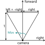
Camera parameters specify a truncated pyramid of view (view frustum), which determines which part of the scene will fall into the final image:
Consider them in turn:
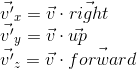
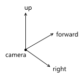
- Местоположение и ориентация камеры в пространстве. Положение, очевидно, просто точка. Описать ориентацию можно различными способами. Я буду использовать так называемую «UVN» систему, т.е. ориентация камеры описывается положением связанной с ней системой координат. Обычно, оси в ней называются u, v и n (поэтому и такое название), но я буду использовать right, up и forward — из этих названий проще понять, чему соответствует каждая ось. Мы будем использовать левостороннюю систему координат.
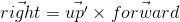
При создании объекта камеры в API можно описывать все три оси — но это очень неудобно для пользователя. Чаще всего, пользователь знает в каком направлении должна смотреть камера, а так же приблизительную ориентацию вектора up (будем называть этот вектор up'). Используя эти два значения мы может построить верную систему координат для камеры по следующему алгоритму:- Вычисляем вектор right используя вектора forward и up' при помощи векторного произведения:
- Теперь вычисляем корректный up, используя rightи forward:

То есть, вектор up' совместно с forward задают плоскость, в которой должен быть расположен настоящий вектор up. Если у вас есть опыт использования OpenGL, то именно по такому алгоритму работает известная функция gluLookAt.
Важно не забыть нормализовать полученные в результате вектора — нам нужна ортонормированная система координат, поскольку ее удобнее использовать в дальнейшем - Вычисляем вектор right используя вектора forward и up' при помощи векторного произведения:
- z-координаты ближней и дальней плоскостей отсечения (near/far clipping plane) в системе координат камеры
- Углы обзора камеры. Они задают размеры усеченной пирамиды обзора:
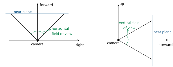
Поскольку сцена в дальнейшем будет спроецирована на плоскость проекции, то изображение на этой плоскости в дальнейшем будет отображено на экране компьютера. Поэтому важно, чтобы соотношение сторон у этой плоскости и окна (или его части), в котором будет показано изображение, совпадали. Этого можно добиться, дав пользователю API возможность задавать только один угол обзора, а второй вычислять в соответствии с соотношением сторон окна. Например, зная горизонтальный угол обзора, мы можем вычислить вертикальный следующим образом: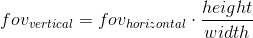
Когда мы обсуждали центральную проекцию, мы видели, что чем дальше находится плоскость проекции от камеры, тем больше размер полученного изображения — мы обозначали расстояние от камеры (считая, что она расположена в начале координат) вдоль оси z до плоскости проекции переменной d. Соответственно, следует решить вопрос, какое значение d нам необходимо выбрать. На самом деле, любое ненулевое. Несмотря на то, что размер изображения увеличивается при увеличении d, пропорционально увеличивается и та часть плоскости проекции, которая пересекается с пирамидой обзора, оставляя одним и тем же масштаб изображения относительно размеров этой части плоскости. В дальнейшем мы будем использовать d = 1 для удобства.
Example in 2D:
As a result, to change the image scale, we need to change the viewing angles - this will change the size of the part of the projection plane intersecting with the viewing pyramid, leaving the projection size the same.
We can move and rotate the camera, changing the position and orientation of its coordinate system. Code example:
Hidden text
void camera::move_right(float distance)
{
	m_position += m_right * distance;
}
void camera::move_left(float const distance)
{
	move_right(-distance);
}
void camera::move_up(float const distance)
{
	m_position += m_up * distance;
}
void camera::move_down(float const distance)
{
	move_up(-distance);
}
void camera::move_forward(float const distance)
{
	m_position += m_forward * distance;
}
void camera::move_backward(float const distance)
{
	move_forward(-distance);
}
void camera::yaw(float const radians)
{
	matrix3x3 const rotation{matrix3x3::rotation_around_y_axis(radians)};
	m_forward = m_forward * rotation;
	m_right = m_right * rotation;
	m_up = m_up * rotation;
}
void camera::pitch(float const radians)
{
	matrix3x3 const rotation{matrix3x3::rotation_around_x_axis(radians)};
	m_forward = m_forward * rotation;
	m_right = m_right * rotation;
	m_up = m_up * rotation;
}
Graphic conveyor
Now we have all the necessary foundation in order to describe in steps the steps that are necessary to obtain an image of a three-dimensional scene on a computer screen. For simplicity, we assume that the pipeline draws one object at a time.
Inbound pipeline parameters:
- Object and its orientation in the world coordinate system
- The camera whose parameters we will use when compiling the image
1. Transition to the world coordinate system
At this stage, we transform the vertices of the object from the local coordinate system to the world.
Assume that the orientation of the object in the world coordinate system is defined by the following parameters:
- At what point in the world coordinate system is the object: (x world , y world , z world )
- How the object is rotated: (r x , r y , r z )
- Object scale: (s x , s y , s z )
We call the matrices of these transformations T , R, and S, respectively. To obtain the final matrix, which will transform the object into a world coordinate system, it is enough for us to multiply them. It is important to note here that the order of matrix multiplication plays a role - this directly follows from the fact that matrix multiplication is non-commutative.
Recall that scaling occurs relative to the origin. If we first move the object to the desired point, and then apply the scale to it, we will get the wrong result - the position of the object will change again after scaling. A simple example:
A similar rule applies to rotation - it occurs relative to the origin, which means the position of the object will change if we first move.
Thus, the correct sequence in our case is as follows: scaling - rotation - displacement:
2. Transition to the camera coordinate system
The transition to the camera coordinate system, in particular, is used to simplify further calculations. In this coordinate system, the camera is located at the origin, and its axes are the vectors forward , right , up , which we examined in the previous section.
The transition to the camera coordinate system consists of two steps:
- We move the world so that the camera position coincides with the origin
- Используя вычисленные оси right, up, forward, вычисляем координаты вершин объекта вдоль этих осей (этот шаг можно рассматривать как поворот системы координат камеры таким образом, чтобы она совпадала с мировой системой координат)
The first step can easily be represented as a displacement matrix by (-pos x , -pos y , -pos z ) , where pos is the position of the camera in the world coordinate system:
To implement the second point, we use the scalar product property, which we considered at the very beginning - the scalar product calculates the projection length along a given axis. Thus, in order to translate point A into the coordinate system of the camera (taking into account the fact that the camera is at the origin - we did this in the first paragraph), we just need to take its scalar product with vectors right , up , forward. We denote the point in the world coordinate system v , and the same point translated into the camera coordinate system, v ' , then:
This operation can be represented as a matrix:
Combining these two transformations, we get the transition matrix to the camera coordinate system:
Schematically, this process can be represented as follows:
3. Transition to a homogeneous clipping space and normalization of coordinates
As a result of the previous paragraph, we got the coordinates of the vertices of the object in the camera coordinate system. The next thing to do is to project these vertices onto a plane and “cut off” the extra vertices. The top of the object is cut off if it lies outside the viewing pyramid (i.e., its projection does not lie on the part of the plane that the viewing pyramid covers). For example, vertex v 1 in the figure below:
Both of these tasks are partially solved by the projection matrix. “Partially” - because it does not produce the projection itself, but prepares w- The vertex coordinate for this. Because of this, the name "projection matrix" does not sound very suitable (although this is a fairly common term), and I will hereinafter call it the clip matrix, since it also maps the truncated viewing pyramid to a homogeneous clipping space (homogeneous clip space).
But first things first. So, the first is preparation for projection. To do this, we put the z- coordinate of the vertex in its w- coordinate. The projection itself (i.e. division by z ) will occur with further normalization of the w-coordinate - i.e. when returning to the space w = 1 .
The next thing this matrix should do is translate the coordinates of the vertices of the object from the camera space into a homogeneous clip space. This is a space in which the coordinates of the non-truncated vertices are such that after applying the projection (i.e., dividing by the w- coordinate, since we saved the old z- coordinate in it), the coordinates of the vertex are normalized, i.e. satisfy the following conditions:
Inequality for z- coordinates may vary for different APIs. For example, in OpenGL it corresponds to what is higher. In Direct3D, the z- coordinate is displayed in the interval [0, 1] . We will use the interval accepted in OpenGL, i.e. [-1, 1] .
Such coordinates are called normalized device coordinates (or simply NDC).
Since we obtain NDC coordinates by dividing the coordinates by w , the vertices in the clipping space satisfy the following conditions:
Thus, by translating the vertices into this space, we can find out whether it is necessary to cut off the vertex by simply checking its coordinates for the inequalities above. Any vertex that does not satisfy these conditions must be cut off. Clipping itself is a topic for a separate article, since its correct implementation leads to the creation of new vertices. So far, as a quick fix, we will not draw a face if at least one of its vertices is cut off. Of course, the result is not very accurate. For example, for a machine model, it looks like this:
Total, this stage consists of the following steps:
- Get the vertices in camera space
- Multiply by the cutoff matrix - go to the cutoff space
- We mark the cut off vertices, checking by the inequalities described above
- Делим координаты каждой вершины на ее w-координату — переходим к нормализованным координатам
Now we will consider how we display the coordinates from the camera space to the clipping space. Recall that we decided to use the projection plane z = 1 . First we need to find a function that displays the coordinates that lie at the intersection of the pyramid of view and the projection plane in the interval [-1, 1] . To do this, find the coordinates of the points that define this part of the plane. These two points have coordinates (left, top) and (right, bottom) . We will consider only the case when the pyramid of view is symmetric with respect to the direction of the camera.
We can calculate them using viewing angles:
We
get : Similarly for top and bottom :
Thus, we need to map the interval [left, right] , [bottom, top] , [near, far] to [-1; 1] . We find a linear function that gives such a result for left and right :
Similarly, we get a function for bottom and top :
The expression for z is found differently. Instead of considering a function of the form az + b, we will consider a function a · 1 / z + b, because in the future, when we implement the depth buffer, we will need to linearly interpolate the inverse of the z-coordinate. We will not consider this issue now, and just take it for granted. We
get : Thus, we can write that the normalized coordinates are obtained as follows from the coordinates in the camera space:
We cannot immediately apply these formulas, because division by z will occur later, when the w coordinate is normalized . We can take advantage of this, and instead calculate the following values (multiplying by z), which, after dividing by w , will result in normalized coordinates:
It is with these formulas that we are transforming into a cutoff space. We can write this transformation in matrix form (additionally remembering that we put z in the w- coordinate ):
Go to screen coordinate system
To the current stage, we have the coordinates of the vertices of the object in NDC. We need to translate them into the screen coordinate system. Recall that the upper left corner of the projection plane was mapped to (-1, 1), and the lower right corner to (1, -1). For the screen, I will use the upper left corner as the origin of the coordinate system, with the axes pointing to the right and down:
This viewport transformation can be done using simple formulas:
Or, in matrix form:
We will leave the use of z ndc until the depth buffer is implemented.
As a result, we have the coordinates of the vertices on the screen, which we use to draw.
Code Implementation
The following is an example code that implements the pipeline using the method described above and performs rendering in wireframe mode (i.e., simply connecting the vertices with lines). It also implies that the object is described by a set of vertices and a set of indices of the vertices (faces) that its polygons consist of:
Hidden text
void pipeline::draw_mesh(
	std::shared_ptr mesh,
	vector3 const& position,
	vector3 const& rotation,
	camera const& camera,
	bitmap_painter& painter) const
{
	matrix4x4 const local_to_world_transform{
		matrix4x4::rotation_around_x_axis(rotation.x) *
		matrix4x4::rotation_around_y_axis(rotation.y) *
		matrix4x4::rotation_around_z_axis(rotation.z) *
		matrix4x4::translation(position.x, position.y, position.z)};
	matrix4x4 const camera_rotation{
		camera.get_right().x, camera.get_up().x, camera.get_forward().x, 0.0f,
		camera.get_right().y, camera.get_up().y, camera.get_forward().y, 0.0f,
		camera.get_right().z, camera.get_up().z, camera.get_forward().z, 0.0f,
		0.0f, 0.0f, 0.0f, 1.0f};
	matrix4x4 const camera_translation{
		1.0f, 0.0f, 0.0f, 0.0f,
		0.0f, 1.0f, 0.0f, 0.0f,
		0.0f, 0.0f, 1.0f, 0.0f,
		-camera.get_position().x, -camera.get_position().y, -camera.get_position().z, 1.0f};
	matrix4x4 const world_to_camera_transform{camera_translation * camera_rotation};
    float const projection_plane_z{1.0f};
	float const near{camera.get_near_plane_z()};
	float const far{camera.get_far_plane_z()};
	float const right{std::tan(camera.get_horizontal_fov() / 2.0f) * projection_plane_z};
	float const left{-right};
	float const top{std::tan(camera.get_vertical_fov() / 2.0f) * projection_plane_z};
	float const bottom{-top};
	matrix4x4 const camera_to_clip_transform{
		2.0f * projection_plane_z / (right - left), 0.0f, 0.0f, 0.0f,
		0.0f, 2.0f * projection_plane_z / (top - bottom), 0.0f, 0.0f,
		(left + right) / (left - right), (bottom + top) / (bottom - top), (far + near) / (far - near), 1.0f,
		0.0f, 0.0f, -2.0f * near * far / (far - near), 0.0f};
	matrix4x4 const local_to_clip_transform{
		local_to_world_transform * world_to_camera_transform * camera_to_clip_transform};
	std::vector transformed_vertices;
	for (vector3 const& v : mesh->get_vertices())
	{
		vector4 v_transformed{vector4{v.x, v.y, v.z, 1.0f} * local_to_clip_transform};
		if ((v_transformed.x > v_transformed.w) || (v_transformed.x < -v_transformed.w))
		{
			mark_vector4_as_clipped(v_transformed);
		}
		else if ((v_transformed.y > v_transformed.w) || (v_transformed.y < -v_transformed.w))
		{
			mark_vector4_as_clipped(v_transformed);
		}
		else if ((v_transformed.z > v_transformed.w) || (v_transformed.z < -v_transformed.w))
		{
			mark_vector4_as_clipped(v_transformed);
		}
		transformed_vertices.push_back(v_transformed);
	}
    float const width{static_cast(painter.get_bitmap_width())};
    float const height{static_cast(painter.get_bitmap_height())};
    matrix4x4 const ndc_to_screen{
            width / 2.0f, 0.0f, 0.0f, 0.0f,
            0.0f, -height / 2.0f, 0.0f, 0.0f,
            0.0f, 0.0f, 1.0f, 0.0f,
            width / 2.0f, height / 2.0f, 0.0f, 1.0f};
	for (vector4& v : transformed_vertices)
	{
		if (is_vector4_marked_as_clipped(v))
		{
			continue;
		}
		float const w_reciprocal{1.0f / v.w};
		v.x *= w_reciprocal;
		v.y *= w_reciprocal;
		v.z *= w_reciprocal;
		v.w = 1.0f;
        v = v * ndc_to_screen;
	}
	for (face const& f : mesh->get_faces())
	{
		vector4 const& v1{transformed_vertices[f.index1]};
		vector4 const& v2{transformed_vertices[f.index2]};
		vector4 const& v3{transformed_vertices[f.index3]};
		bool const v1_clipped{is_vector4_marked_as_clipped(v1)};
		bool const v2_clipped{is_vector4_marked_as_clipped(v2)};
		bool const v3_clipped{is_vector4_marked_as_clipped(v3)};
		if (!v1_clipped && !v2_clipped)
		{
			painter.draw_line(
				point2d{static_cast(v1.x), static_cast(v1.y)},
				point2d{static_cast(v2.x), static_cast(v2.y)},
				color{255, 255, 255});
		}
		if (!v3_clipped && !v2_clipped)
		{
			painter.draw_line(
				point2d{static_cast(v2.x), static_cast(v2.y)},
				point2d{static_cast(v3.x), static_cast(v3.y)},
				color{255, 255, 255});
		}
		if (!v1_clipped && !v3_clipped)
		{
			painter.draw_line(
				point2d{static_cast(v3.x), static_cast(v3.y)},
				point2d{static_cast(v1.x), static_cast(v1.y)},
				color{255, 255, 255});
		}
	}
}
SDL2 implementation example
In this section, I will briefly describe how SDL2 can be used to implement rendering.
Initialization, texture creation
The first is, of course, initializing the library and creating the window. If only graphics are needed from the SDL, then you can initialize with the SDL_INIT_VIDEO flag :
Hidden text
if (SDL_Init(SDL_INIT_VIDEO) < 0)
{
	throw std::runtime_error(SDL_GetError());
}
m_window = SDL_CreateWindow(
	"lantern",
	SDL_WINDOWPOS_UNDEFINED, SDL_WINDOWPOS_UNDEFINED,
	width, height,
	SDL_WINDOW_SHOWN);
if (m_window == nullptr)
{
	throw std::runtime_error(SDL_GetError());
}
m_renderer = SDL_CreateRenderer(m_window, -1, SDL_RENDERER_ACCELERATED);
if (m_renderer == nullptr)
{
	throw std::runtime_error(SDL_GetError());
}
Then, create a texture into which we will draw. I will use the ARGB8888 format , which means that 4 bytes will be allocated for each pixel in the texture - three bytes for RGB channels, and one for alpha channel.
Hidden text
m_target_texture = SDL_CreateTexture(
	m_renderer,
	SDL_PIXELFORMAT_ARGB8888,
	SDL_TEXTUREACCESS_STREAMING,
	width, height);
if (m_target_texture == nullptr)
{
	throw std::runtime_error(SDL_GetError());
}
We must not forget to “clear” the SDL and all the variables taken from it when the application exits:
Hidden text
if (m_target_texture != nullptr)
{
	SDL_DestroyTexture(m_target_texture);
	m_target_texture = nullptr;
}
if (m_renderer != nullptr)
{
	SDL_DestroyRenderer(m_renderer);
	m_renderer = nullptr;
}
if (m_window != nullptr)
{
	SDL_DestroyWindow(m_window);
	m_window = nullptr;
}
SDL_Quit();
Drawing, displaying on the screen
We can use SDL_UpdateTexture to update the texture, which we then display on the screen. This function accepts, among others, the following parameters:
- Data is an array of bytes, which is an array of pixels with corresponding values
- The number of bytes in one line of the image (pitch) is calculated as the number of pixels times 4 (because the format is ARGB8888 )
It is logical to separate the drawing functionality into a texture represented by an array of bytes into a separate class. It will allocate memory for the array, clear the texture, draw pixels and lines. Drawing a pixel can be done as follows (byte order varies depending on SDL_BYTEORDER ):
Hidden text
void bitmap_painter::draw_pixel(point2d const& point, color const& c)
{
	unsigned int const pixel_first_byte_index{m_pitch * point.y + point.x * 4};
#if SDL_BYTEORDER == SDL_BIG_ENDIAN
	m_data[pixel_first_byte_index + 0] = c.b;
	m_data[pixel_first_byte_index + 1] = c.g;
	m_data[pixel_first_byte_index + 2] = c.r;
	// m_data[pixel_first_byte_index + 3] is alpha, we don't use it for now
#else
	// m_data[pixel_first_byte_index + 0] is alpha, we don't use it for now
	m_data[pixel_first_byte_index + 1] = c.r;
	m_data[pixel_first_byte_index + 2] = c.g;
	m_data[pixel_first_byte_index + 3] = c.b;
#endif
}
Line drawing can be implemented, for example, according to the Bresenham algorithm .
After using SDL_UpdateTexture , you need to copy the texture to SDL_Renderer and display it using SDL_RenderPresent . Together:
Hidden text
SDL_UpdateTexture(m_target_texture, nullptr, m_painter.get_data(), m_painter.get_pitch());
SDL_RenderCopy(m_renderer, m_target_texture, nullptr, nullptr);
SDL_RenderPresent(m_renderer);
That's all. Link to the project: https://github.com/loreglean/lantern .