We develop the NIOS II processor module for IDA Pro

IDA Pro Disassembler Interface Screenshot

IDA Pro is a famous disassembler that information security researchers around the world have been using for many years. We at Positive Technologies also use this tool. Moreover, we managed to develop our own disassembler processor module for the microprocessor architecture of NIOS II , which improves the speed and convenience of code analysis.

Today I will talk about the history of this project and show you what happened in the end.

Prehistory

It all started in 2016, when we had to develop our own processor module to analyze the firmware in one task. Development was carried out from scratch according to the manual of the Nios II Classic Processor Reference Guide , which was then the most relevant. In total, this work took about two weeks.

The processor module was developed for version IDA 6.9. IDA Python was chosen for speed. In the place where the processor modules live, the subdirectory procs inside the IDA Pro installation directory, there are three modules in Python: msp430, ebc, spu. They can see how the module is arranged and how the basic disassembling functionality can be implemented:

• parsing instructions and operands,
• simplifying and displaying them,
• creating offsets, cross references, as well as the code and data to which they refer,
• processing switch constructions
• handling of stack manipulations and stack variables.

Approximately this functionality was implemented at that time. Fortunately, the tool came in handy in the process of working on another task, during which, a year later, it was actively used and refined.

I decided to share the experience of creating a processor module with the community at the PHDays 8 conference. The presentation aroused interest (the video of the report was published on the PHDays website), even the creator of IDA Pro Ilfak Gilfanov attended it. One of his questions was whether support for IDA Pro version 7 was implemented. At that time it was not there, but after the speech I promised to make the appropriate release of the module. This is where the fun began.

Now the most recent is the manual from Intelwhich was used to verify and check for errors. I have significantly reworked the module, added a number of new features, including solving the problems that previously could not be won. And, of course, added support for the 7th version of IDA Pro. That's what happened.

NIOS II software model

NIOS II is a software processor developed for Altera FPGAs (now part of Intel). From the point of view of programs, it has the following features: byte order little endian, 32-bit address space, 32-bit instruction set, i.e., 4 bytes are fixed, 32 general registers and 32 special purposes are used for encoding each command.

Disassembling and Code References

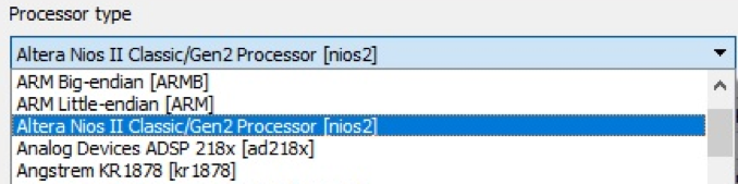
So, we have opened a new file in IDA Pro, with firmware for NIOS II processor. After installing the module, we will see it in the list of IDA Pro processors. The choice of processor is presented in the figure.



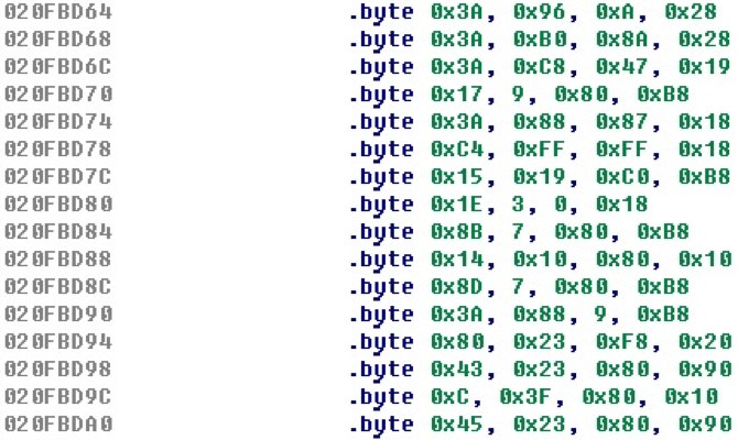
Suppose that the module has not yet implemented even basic command parsing. Given that each command takes 4 bytes, we group bytes by four, then everything will look something like this.



After implementing the basic functionality of decoding instructions and operands, displaying them, and analyzing control transfer instructions, the set of bytes from the example above is converted to the following code.



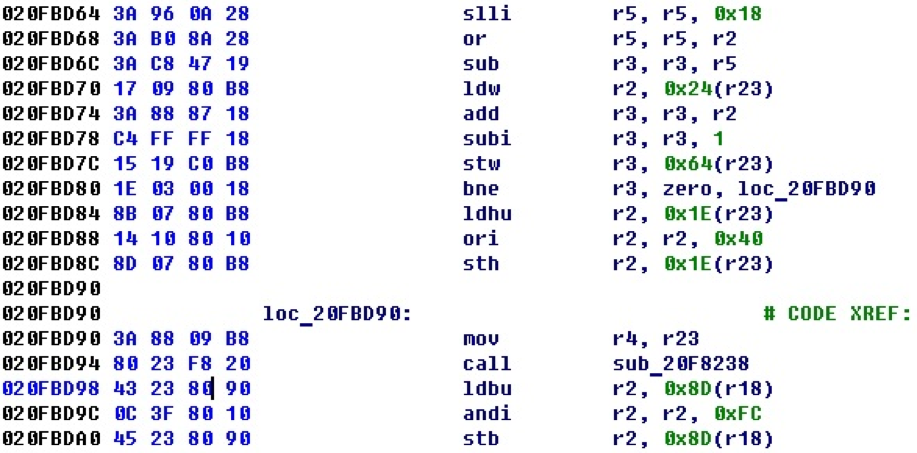
As you can see from the example, cross-references are also formed from the control transfer commands (in this case, you can see the conditional transition and the procedure call).

One of the useful properties that can be implemented in the processor modules is the comments to the commands. If you turn off the output of byte values ​​and enable the display of comments, the same piece of code will already look like this.



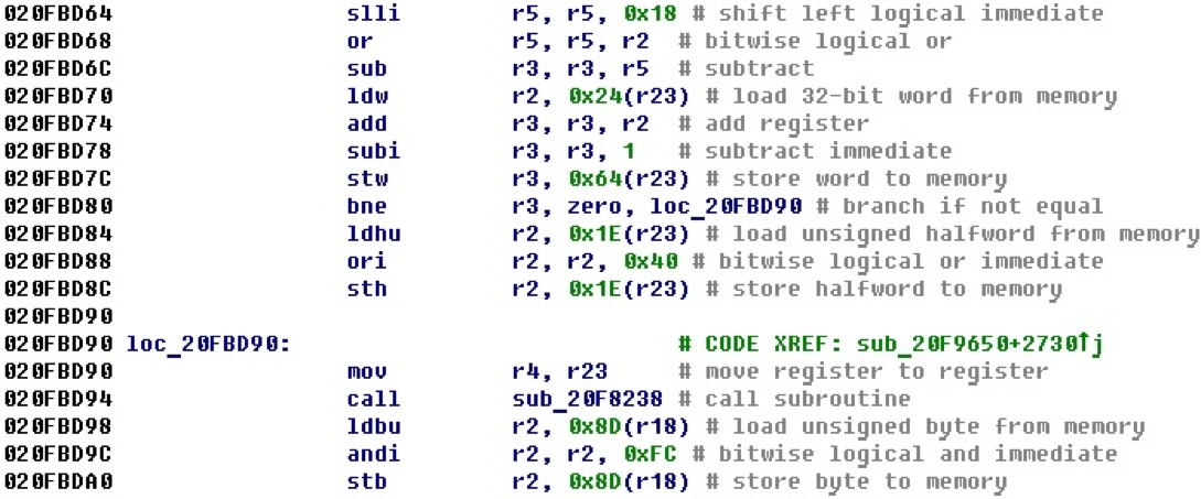
Here, if you first come across an assembler code of a new architecture for you, you can understand what is happening with the help of comments. Further, the code examples will be in the same form - with comments, so as not to look at the NIOS II manual, but to immediately understand what is happening in the section of the code that is given as an example.

Pseudoinstructions and command simplification

Some of the NIOS II commands are pseudoinstructions. For such teams there are no separate opcodes, and they are modeled as special cases of other teams. In the disassembly process, instructions are simplified — replacing certain combinations with pseudoinstructions. Pseudoinstructions in NIOS II can generally be divided into four types:

• when one of the sources is zero (r0) and can be removed from consideration,
• when there is a negative value in the command and the command is replaced with the opposite,
• when the condition is replaced with the opposite,
• when the 32-bit offset is entered in two teams in parts (junior and senior) and this is replaced by one command.

The first two types have been implemented, since the replacement of the condition does not give much, and the 32-bit offsets have more options than the ones presented in the manual.

For example, for the first view, consider the code.



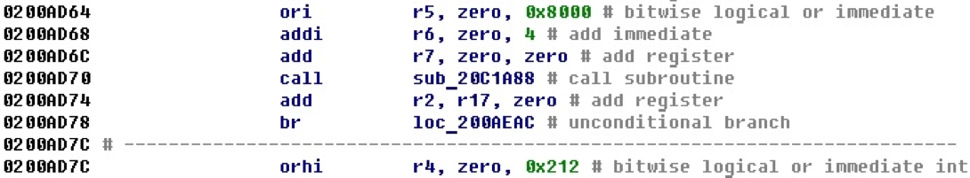
It can be seen that the use of the zero register in calculations is often found here. If you look closely at this example, you will notice that all commands except the transfer of control are variants of simply entering values ​​into certain registers.

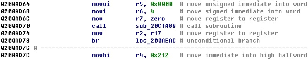
After implementing the processing of pseudoinstructions, we get the same piece of code, but now it looks more readable, and instead of variations of the or and add commands, we get the variations of the mov command.

Stack variables

The NIOS II architecture supports the stack, and in addition to the stack pointer sp, there is also a pointer to the stack frame fp. Consider an example of a small procedure that uses a stack.



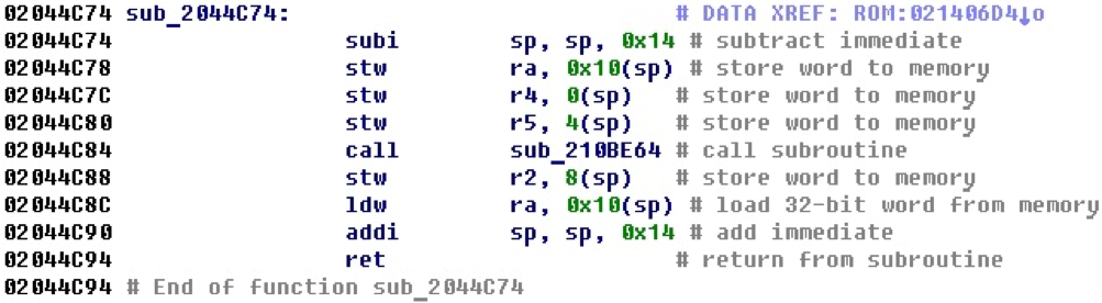
Obviously, space is allocated on the stack for local variables. It can be assumed that the register ra is stored in the stack variable, and then restored from it.

After adding functionality to the module that tracks changes to the stack pointer and creates stack variables, the same example will look like this.



Now the code looks a little clearer, and it is already possible to name the stack variables and parse their purpose, following the cross-references. The function in the example is of type __fastcall and its arguments in registers r4 and r5 are put on the stack to call a subroutine that is of type _stdcall.

32-bit numbers and offsets

The peculiarity of NIOS II is that in one operation, that is, when executing one command, you can, as a maximum, enter a direct value of 2 bytes (16 bits) into the register. On the other hand, the processor registers and address space are 32-bit, that is, for addressing in the register, 4 bytes must be added.

To solve this problem, two-part displacements are used. A similar mechanism is used in processors in PowerPC: the offset consists of two parts, the highest and the lowest, and is entered in the register by two commands. In PowerPC, it looks like this.



In this approach, cross-references are formed from both teams, although in fact the adjustment to the address occurs in the second command. This can sometimes cause inconvenience when counting the number of cross-references.

In the offset properties, the non-standard type HIGHA16 is used for the higher part, the type HIGH16 is sometimes used, and the lower part - LOW16.



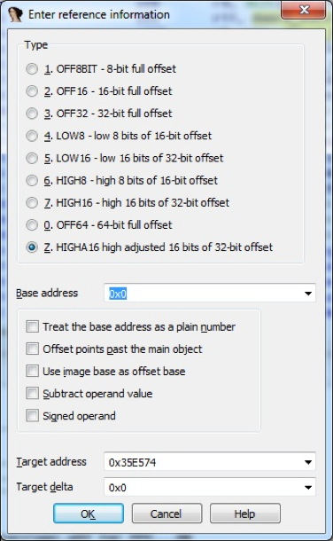
In the calculation of 32-bit numbers from two parts there is nothing complicated. Difficulties arise in the formation of operands as offsets for two separate commands. All this processing falls on the processor module. There are no examples of how to implement this (especially in Python) in the IDA SDK.

In the report at PHDays, the displacements stood as an unsolved problem. To solve the problem, we cheated: 32-bit offset only from the younger part - on the base. The base is calculated as the highest part shifted to the left by 16 bits.



With this approach, a cross reference is formed only from the command for entering the lower part of the 32-bit offset.

The base properties are visible in the offset properties, and the property is marked in order to treat it as a number, so that a large number of cross-references to the address itself, which is accepted as a base, are not formed.



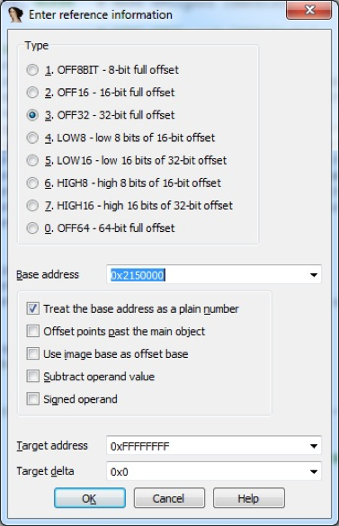
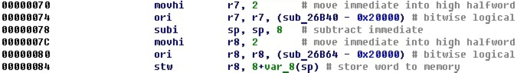
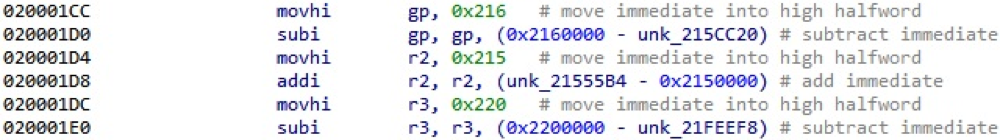
The code for NIOS II contains the following mechanism for inserting 32-bit numbers into a register. First, the upper part of the offset is entered into the register with the movhi command. Then the younger part joins her. This can be done in three ways (commands): addition addi, subtraction subi, logical OR ori.

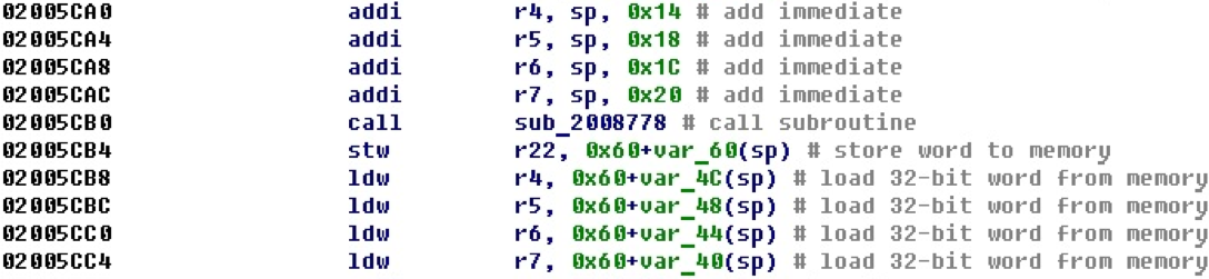
For example, in the next section of the code, the registers are set to 32-bit numbers, which are then entered into registers — arguments before the function call.



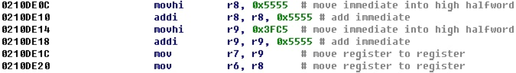
After adding the calculation of offsets, we get the following representation of this block of code.



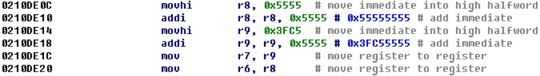
The resulting 32-bit offset is displayed next to the entry command for its lowest part. This example is quite visual, and we could even easily calculate all 32-bit numbers in our mind just by attaching the lower and upper parts. Judging by the values, most likely, they are not offsets.

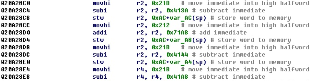
Consider the case when subtraction is used when entering the younger part. In this example, to determine the final 32-bit numbers (offsets) on the move will not work.



After applying the calculation of 32-bit numbers we get the following form.



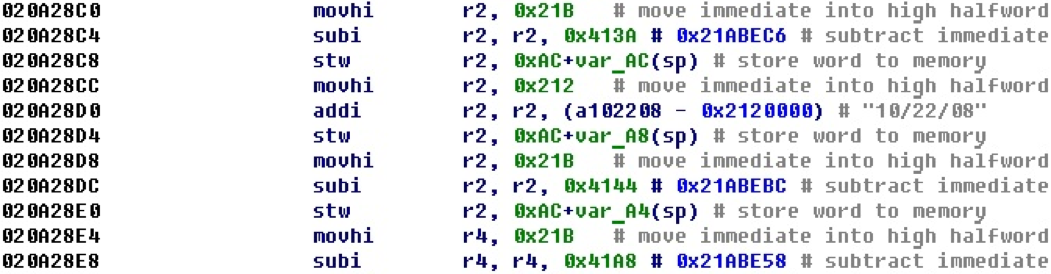
Here we see that now, if the address is in the address space, an offset is formed on it, and the value that was formed as a result of the junior and senior parts is not displayed next to it. Here we get an offset to the string "10/22/08". In order for the remaining offsets to point to valid addresses, increase the segment a little.



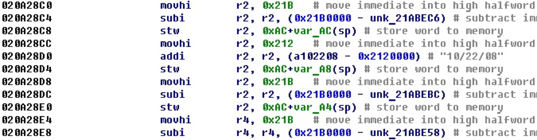
After increasing the segment, we find that now all the calculated 32-bit numbers are offsets and point to valid addresses.

It was mentioned above that there is another option for calculating offsets when the logical OR command is used. Here is an example code where two offsets are calculated this way.



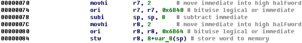
That, which is calculated in the register r8, is then pushed onto the stack.

After the conversion, it is clear that in this case the registers are set to the addresses of the beginning of the procedures, that is, the address of the procedure is put on the stack.

Reading and writing relative to the base

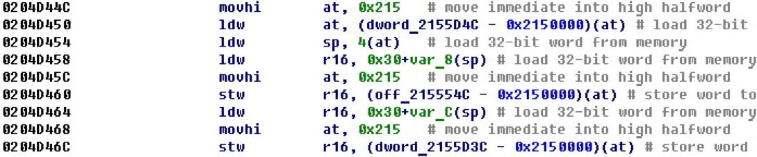
Before that, we considered cases when a 32-bit number entered using two commands could be just a number and also an offset. In the following example, the base is entered into the upper part of the register, then a read or write occurs relative to it.



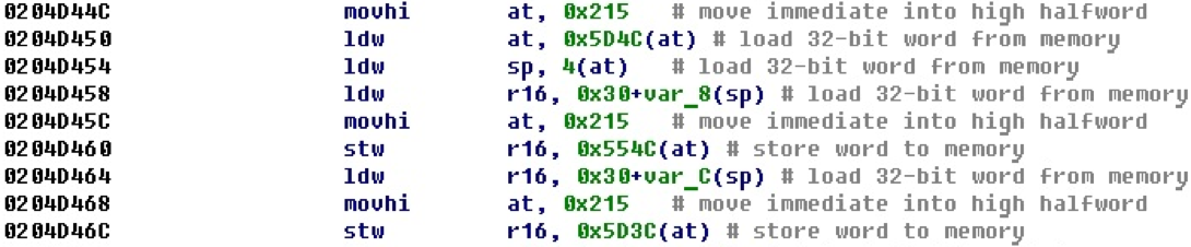
After processing such situations, we obtain offsets for variables from the read and write commands themselves. At the same time, depending on the dimension of the operation, the size of the variable itself is set.

Switch constructions

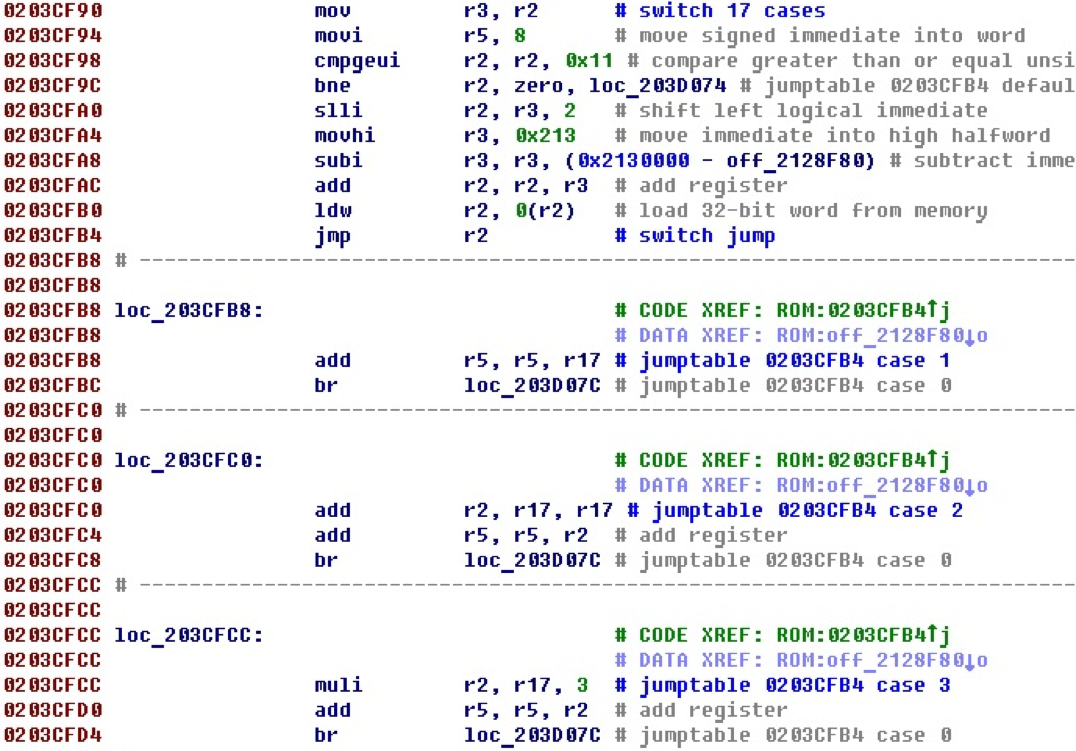
The switch constructions met in binary files can facilitate the analysis. For example, according to the number of choices made inside the switch construction, it is possible to localize a switch responsible for processing some protocol or set of commands. Therefore, there is the task of recognizing the switch itself and their parameters. Consider the following code snippet.



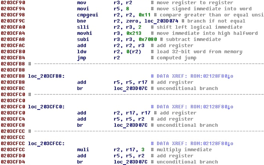
The execution flow stops at the jmp r2 register transition. Next come the code blocks that are referenced from the data, and at the end of each block there is a jump to the same label. Obviously, this is a switch construction and these separate blocks handle specific cases from it. Above, you can also see the check of the number of cases and the default jump.

After adding the switch processing, this code will look like this.



Now the jump itself is indicated, the address of the table with offsets, the number of cases, as well as each case with the corresponding number.

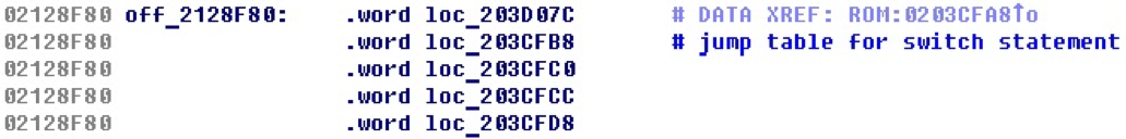
The table itself with offsets to the options is as follows. To save space, the first five elements are given.



In essence, the switch processing is to go back through the code and search for all its components. That is, a certain organization of the switch is described. Sometimes there may be exceptions in the diagrams. This may be the reason for cases when seemingly visual switches are not recognized in existing processor modules. It turns out that the real switch simply does not fall under the scheme, which is defined inside the processor module. There are still possible options when the scheme seems to be there, but inside it there are still other commands not participating in the scheme, or the main commands are swapped, or it is broken by transitions.

The NIOS II processor module recognizes a switch with such "extraneous" instructions between the main commands, as well as with the rearranged main commands and with transitions that break the circuit. A reverse pass through the execution path is used, taking into account possible transitions that break the circuit, with the installation of internal variables that signal different states of the recognizer. As a result, about 10 different options for the organization of switch, found in the firmware, are recognized.

Instructions custom

There is an interesting feature in the NIOS II architecture - the custom instruction. It gives access to 256 user-definable instructions that are possible in the NIOS II architecture. In its work, in addition to general-purpose registers, the custom instruction can refer to a special set of 32 custom registers. After implementing the custom command parsing logic, we get the following view.



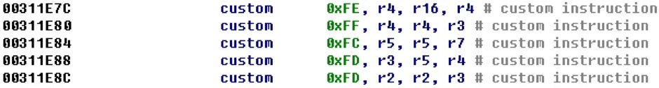
You may notice that the last two instructions have the same instruction number and seem to perform the same actions.

According to the instructions custom there is a separate manual. According to him, one of the most complete and modern versions of the custom instruction set is the NIOS II Floating Point Hardware 2 Component (FPH2) instruction set for working with floating point. After implementing the FPH2 command parsing, the example will look like this.



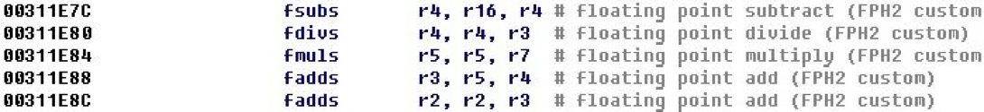
On the mnemonic of the last two teams, we are convinced that they really perform the same action - the fadds command.

Jumps by register value

In the studied firmwares, there is often a situation when a jump is performed on the register value, into which a 32-bit offset is entered before it, defining the place of the jump.

Consider a piece of code.



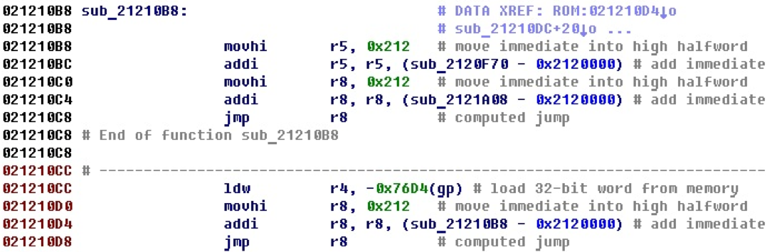
In the last line there is a jump on the register value, while it is clear that the address of the procedure that begins in the first line of the example is entered into the register first. In this case, it is obvious that the jump takes place at its beginning.

After adding the jump recognition functionality, we get the following view.



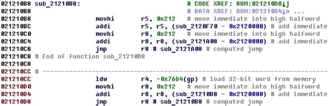
Next to the jmp r8 command is the address where the jump occurs, if it was possible to calculate it. Also formed a cross-reference between the team and the address where the jump occurs. In this case, the link is visible in the first line, the jump itself is performed from the last line.

Register value gp (global pointer), save and load

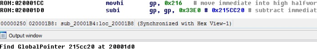
It is common to use a global pointer that is configured for an address, and relative to it, the variables are addressed. In NIOS II, the global pointer register is used to store the global pointer. At a certain point, as a rule, in the initialization procedures of the firmware, the value of the address is entered into the gp register. The processor module handles this situation; To illustrate this, the following are code samples and an IDA Pro output window with debug messages enabled in the processor module.

In this example, the processor module finds and calculates the value of the gp register in the new database. When closing the idb base, the gp value is stored in the base.



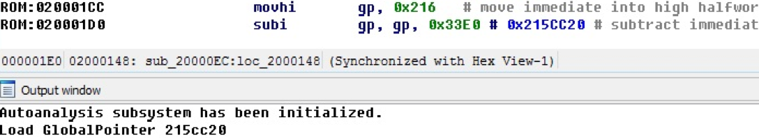
When loading an already existing idb base and if the gp value has already been found, it is loaded from the base, as shown in the debugging message in the following example.

Read and write relative to gp

Common operations are reading and writing with an offset from the gp register. For example, the following example performs three reads and one write of this type.



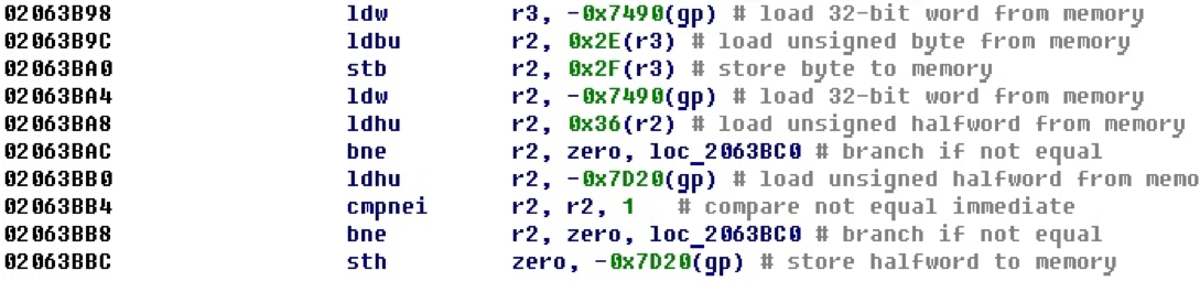
Since the value of the address, which is stored in the register gp, we have already received, it is possible to address this kind of reading and writing.

After adding the processing of read and write situations relative to the gp register, we obtain a more convenient picture.



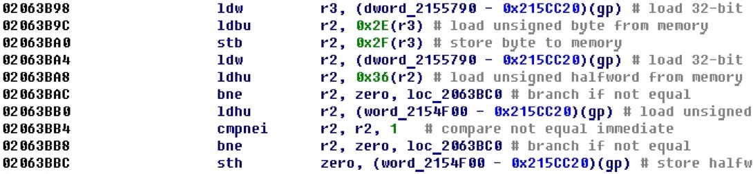
Here you can see which variables are addressed, track their use and identify their purpose.

Gp addressing

There is another use of the gp register for addressing variables.



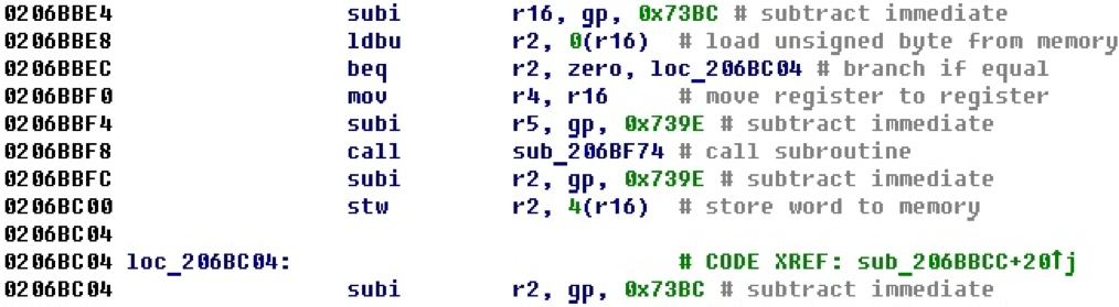
For example, here we see that registers are configured relative to the gp register to some variables or data areas.

After adding functionality that recognizes such situations, which transforms into offsets and adds cross-references, we get the following form.



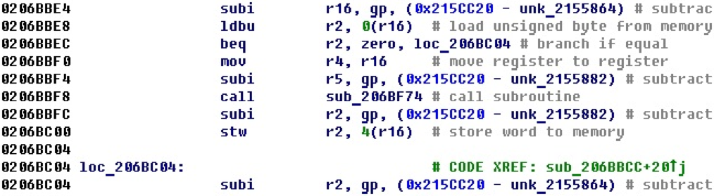
Here you can already see on which areas registers are configured for gp, and it becomes clearer what is happening.

Addressing relatively sp

Similarly, in the following example, the registers are tuned to some memory areas, this time relative to the sp - stack pointer register.



Obviously, the registers are tuned to some local variables. Such situations — setting arguments to local buffers before procedure calls — are quite common.

After adding processing (converting immediate values ​​to offsets), we obtain the following form.



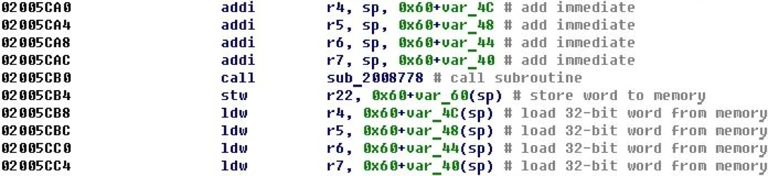
Now it becomes clear that after calling the procedure, the values ​​are loaded from those variables whose addresses were passed as parameters before the function call.

Cross references from code to structure fields

Defining structures and using them in IDA Pro can facilitate code analysis.



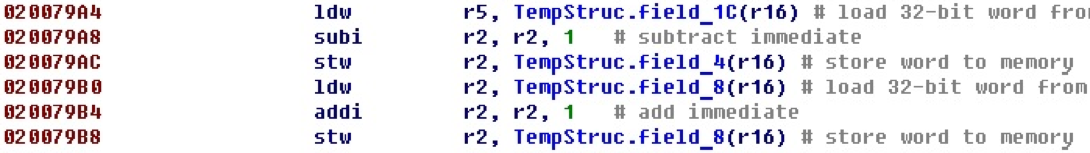
Looking at this section of the code, one can understand that the field field_8 is incremented and, possibly, is the counter of the occurrence of any event. If the reading and writing fields are separated in the code at a great distance, cross-references can help in the analysis.

Consider the structure itself.



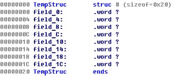
Although, as you can see, there are no references to the fields of the structures from the code to the elements of the structures.

After such situations are handled, for our case everything will look like this.



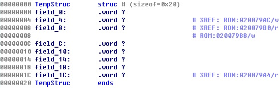
Now there are cross-references to the fields of structures from specific commands that work with these fields. Forward and backward cross references are created, and you can track through different procedures, where the values ​​of the structure fields are read and where they are entered.

Discrepancies between the manual and reality

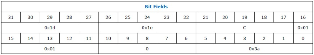
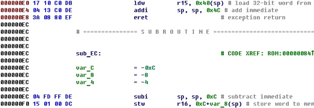
In the manual when decoding some commands certain bits must take strictly defined values. For example, for the return command from an eret exception, bits 22-26 should be 0x1E.



Here is an example of this command from a single firmware.



Opening another firmware in a place with a similar context, we meet a different situation.



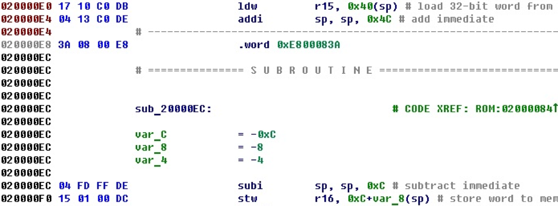
These bytes are not automatically converted into a command, although there is processing of all commands. Judging by the environment, and even a similar address, it must be the same team. Let's look carefully at the bytes. This is the same eret command, with the exception that bits 22-26 are not equal to 0x1E, but equal to zero.

It is necessary to correct a little analysis of this command. Now it is not quite the manual, but true.

IDA 7 support

Beginning with IDA 7.0, the API provided by IDA Python for regular scripts has changed quite a lot. As for the processor modules, the changes are colossal. Despite this, the NIOS II processor module managed to be remade to version 7, and it successfully worked in it.



The only incomprehensible point: when loading a new binary file under NIOS II in IDA 7, the initial automatic analysis that is present in IDA 6.9 does not occur.

Conclusion

In addition to the basic disassembly functionality, examples of which are in the SDK, the processor module has many different features that facilitate the work of the code researcher. It is clear that all this can be done manually, but, for example, when there are thousands and tens of thousands of displacements of different types on a binary file with firmware of a size of a couple of megabytes - why waste time on it? Let the processor module do it for us. After all, how pleasant the possibility of quick navigation through the code under study with the help of cross references helps! This makes IDA such a convenient and enjoyable tool as we know it.

Author : Anton Dorfman, Positive Technologies