Speech Recognition for Dummies

In this article I want to consider the basics of such an interesting area of ​​software development as Speech Recognition. Naturally, I am not an expert in this topic, so my story will be replete with inaccuracies, errors and disappointments. However, the main goal of my “work”, as the name implies, is not a professional analysis of the problem, but a description of the basic concepts, problems and their solutions. In general, I ask all those who are interested welcome under the cat!

Prologue

To begin with, our speech is a sequence of sounds. Sound, in turn, is a superposition (superposition) of sound vibrations (waves) of various frequencies. The wave, as we know from physics, is characterized by two attributes - amplitude and frequency. In order to save the audio signal on a digital medium, it is necessary to divide it into many gaps and take some “average” value on each of them. In this way, mechanical vibrations turn into a set of numbers suitable for processing on modern computers. It follows that the task of speech recognition is reduced to "matching" the set of numerical values ​​(digital signal) and words from a dictionary (Russian language, for example).











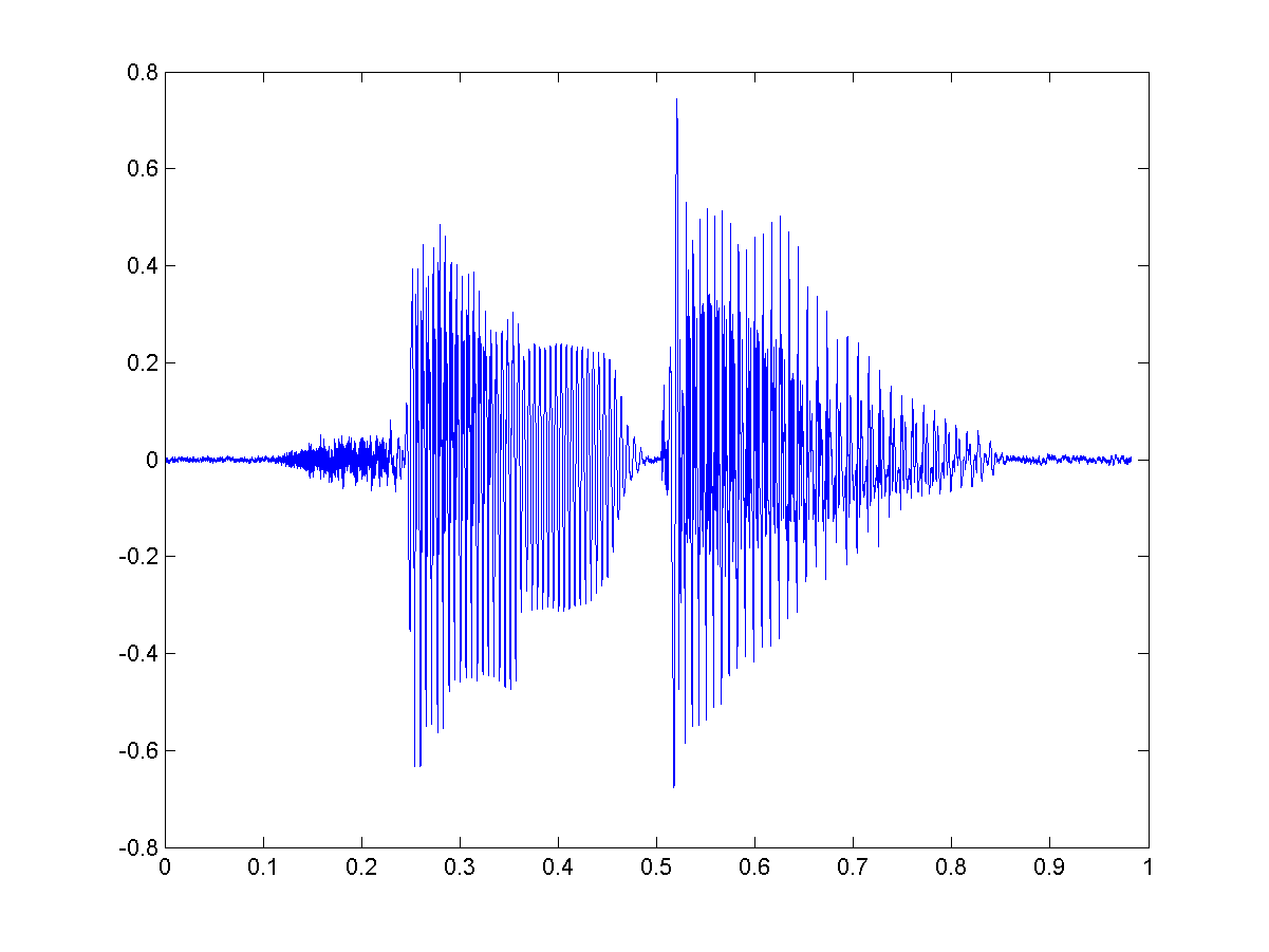
Let's see how, in fact, this very “comparison” can be realized.

Input data

Let's say we have some file / stream with audio data. First of all, we need to understand how it works and how to read it. Let's look at the easiest option - a WAV file. The format implies the presence of two blocks in the file. The first block is a header with information about the audio stream: bitrate, frequency, number of channels, file length, etc. The second block consists of “raw” data - that same digital signal, a set of amplitudes. The logic of reading data in this case is quite simple. We read the header, check some restrictions (lack of compression, for example), save the data in a specially allocated array. An example .

Recognition

Purely theoretically, now we can compare (element by element) our existing sample with some other one, the text of which we already know. That is, try to "recognize" the speech ... But it’s better not to do this :)

Our approach should be stable (well, at least a little) to change the timbre of the voice (the person pronouncing the word), the volume and speed of pronunciation. By element-wise comparison of two audio signals, this, of course, cannot be achieved.

Therefore, we will go in a slightly different way.

Frames

First of all, we’ll break our data into small time frames - frames. Moreover, the frames should not go strictly one after another, but “overlap”. Those. the end of one frame should intersect with the beginning of another.

Frames are a more suitable unit of data analysis than specific signal values, since it is much more convenient to analyze waves at a certain interval than at specific points. The location of the overlapping frames allows smoothing the results of the analysis of frames, turning the idea of ​​frames into a certain “window” moving along the original function (signal values).

It was experimentally established that the optimal frame length should correspond to a gap of 10ms, “overlap” - 50%. Considering that the average word length (at least in my experiments) is 500ms - this step will give us approximately 500 / (10 * 0.5) = 100 frames per word.

Word breaking

The first task that has to be addressed in speech recognition is to break this speech into separate words. For simplicity, suppose that in our case speech contains some pauses (intervals of silence), which can be considered as “separators” of words.

In this case, we need to find some value, the threshold - the values ​​above which are a word, below - silence. There may be several options:

• set with a constant (it will work if the original signal is always generated under the same conditions, in the same way);
• Cluster the signal values, clearly highlighting the set of values ​​corresponding to silence (only works if silence occupies a significant part of the original signal);
• analyze entropy;

As you may have guessed, we will now discuss the last point :) To begin with, entropy is a measure of disorder, “a measure of the uncertainty of any experience” (c). In our case, entropy means how much our signal “fluctuates” within a given frame.

In order to calculate the entropy of a particular frame, perform the following steps:

• suppose that our signal is normalized and all its values ​​lie in the range [-1; 1];
• construct a histogram (distribution density) of the frame signal values:

we calculate the entropy as ;



An example .

And so, we got the value of entropy. But this is just another characteristic of the frame, and in order to separate the sound from the silence, we still need to compare it with something. Some articles recommend taking the entropy threshold equal to the average between its maximum and minimum values ​​(among all frames). However, in my case, this approach did not give any good results.
Fortunately, entropy (in contrast to the same mean square of values) is a relatively independent value. Which allowed me to choose the value of its threshold in the form of a constant (0.1).

Nevertheless, the problems do not end there :( Entropy can sag in the middle of a word (in vowels), or it can suddenly jump up due to a little noise. In order to deal with the first problem, one has to introduce the concept of “minimum distance between words” and “glue” close to lying sets of frames, separated due to subsidence. The second problem is solved by using the “minimum word length” and cutting off all candidates who have not passed the selection (and not used in the first paragraph).

If the speech is not in principle “articulate ", you can try to break the original set of frames into prepared subsequences in a certain way, each of which will be subjected to recognition. But this is a completely different story :)

Mfcc

And so, we have a set of frames corresponding to a certain word. We can follow the path of least resistance and use the mean square of all its values ​​(Root Mean Square) as a numerical characteristic of the frame. However, such a metric carries very little information suitable for further analysis.

This is where Mel-frequency cepstral coefficients come into play. According to Wikipedia (which, as you know, does not lie) MFCC is a kind of representation of the energy of the signal spectrum. The advantages of its use are as follows:

• The signal spectrum is used (that is, the expansion along the basis of orthogonal [co] sinusoidal functions), which allows us to take into account the wave “nature” of the signal during further analysis;
• The spectrum is projected onto a special mel-scale , making it possible to single out the frequencies most significant for human perception;
• The number of calculated coefficients can be limited by any value (for example, 12), which allows you to “compress” the frame and, as a result, the amount of processed information;

Let's look at the process of calculating the MFCC coefficients for a certain frame.

We represent our frame as a vector , where N is the frame size.

Fourier expansion

First of all, we calculate the signal spectrum using the discrete Fourier transform (preferably with its “fast” FFT implementation). It is also recommended to apply the Hamming window function to the obtained values ​​in order to “smooth out” the values ​​at the borders of the frames. That is, the result will be a vector of the following form: It is important to understand that after this transformation along the X axis we have the frequency (hz) of the signal, and along the Y axis we have magnitude (as a way to get away from complex values):

Calculation of mel filters

Let's start with what mel is. Again, according to Wikipedia, mel is a “psychophysical unit of pitch” based on subjective perception by average people. It depends primarily on the frequency of sound (as well as on volume and timbre). In other words, this value shows how much sound of a certain frequency is “significant” for us.

The frequency can be converted to chalk using the following formula (remember it as “formula-1”): The inverse transformation looks like this (remember it as “formula-2”): Mel / frequency graph:








But back to our task. Let's say we have a frame with a size of 256 elements. We know (from the data on the audio format) that the sound frequency in this frame is 16000hz. Suppose that human speech lies in the range from [300; 8000] hz. The number of desired chalk coefficients is set M = 10 (recommended value).

In order to decompose the spectrum obtained above on the mel-scale, we need to create a “comb” of filters. In fact, each mel-filter is a triangular window function , which allows you to sum the amount of energy over a certain frequency range and thereby obtain a mel-coefficient. Knowing the number of chalk coefficients and the analyzed frequency range, we can build a set of such filters:



Please note that the higher the number of the chalk factor, the wider the base of the filter. This is due to the fact that the division of the frequency range of interest to us into the ranges processed by the filters occurs on the chalk scale.

But again we got distracted. And so for our case, the range of frequencies of interest to us is [300, 8000]. According to formula-1, on the chalk scale this range turns into [401.25; 2834.99].

Further, in order to build 10 triangular filters, we need 12 reference points:

m [i] = [401.25, 622.50, 843.75, 1065.00, 1286.25, 1507.50, 1728.74, 1949.99, 2171.24, 2392.49, 2613.74, 2834.99]

Note that on the chalk scale the points are evenly spaced. We translate the scale back to Hertz using formula-2:

h [i] = [300, 517.33, 781.90, 1103.97, 1496.04, 1973.32, 2554.33, 3261.62, 4122.63, 5170.76, 6446.70, 8000]

As you can see now the scale began to gradually stretch, thereby leveling the dynamics of the growth of “significance” at low and high frequencies.

Now we need to superimpose the resulting scale on the spectrum of our frame. As we remember, on the X axis we have the frequency. The length of the spectrum is 256 elements, while it fits in 16000hz. Having solved a simple proportion, you can get the following formula:

f (i) = floor ((frameSize + 1) * h (i) / sampleRate)

which in our case is equivalent

f (i) = 4, 8, 12, 17, 23, 31, 40, 52, 66, 82, 103, 128

That's all! Knowing the reference points on the X-axis of our spectrum, it is easy to construct the filters we need using the following formula:

Application of filters, logarithm of spectrum energy

The use of a filter consists in pairwise multiplication of its values ​​with the values ​​of the spectrum. The result of this operation is the mel factor. Since we have M filters, there will be as many coefficients. However, we need to apply mel filters not to the spectrum values, but to its energy. Then prologarithm the results. It is believed that in this way the sensitivity of the coefficients to noise is reduced.

Cosine transform

The discrete cosine transform (DCT) is used to obtain the same “cepstral" coefficients. Its meaning is to “squeeze” the results obtained, increasing the significance of the first coefficients and decreasing the significance of the latter.

In this case, DCTII is used without any scale factor multiplication . Now, for each frame, we have a set of M mfcc coefficients that can be used for further analysis. Sample code for the upstream methods can be found here .

Recognition algorithm

Here, dear reader, the main disappointment awaits you. On the Internet, I happened to see a lot of highly intellectual (and not so) disputes about which method of recognition is better. Someone advocates for Hidden Markov Models, some advocates for neural networks, someone’s thoughts can’t be understood in principle :)

In any case, a lot of preferences are given to SMM , and I’m going to add their implementation to my code ... in the future: )

At the moment, I propose to dwell on a much less effective, but at times simpler way.

And so, remember that our task is to recognize a word from some dictionary. For simplicity, we will recognize the names of the first ten digits: “one“, “two“, “three“, “four“, “five“, “six“, “seven“, “eight“, “nine“, “ten“.

Now let's pick up an iPhone / Android and go through L colleagues asking them to dictate these words for the record. Next, we associate (in some local database or simple file) each word L with the sets of mfcc coefficients of the corresponding records.

We will call this correspondence “Model”, and the process itself - Machine Learning! In fact, simply adding new samples to the database has an extremely weak connection with machine learning ... But the term is fashionable :)

The task now is to select the “closest” model for a certain set of mfcc coefficients (a recognizable word). At first glance, the problem can be solved quite simply:

• for each model we find the average (Euclidean) distance between the identified mfcc vector and the model vectors;
• choose the model that is correct, the average distance to which will be the smallest;

However, the same word can be pronounced both by Andrei Malakhov and some of his Estonian counterparts. In other words, the size of the mfcc vector for the same word can be different.

Fortunately, the task of comparing sequences of different lengths has already been solved in the form of a Dynamic Time Warping algorithm. This dynamic programming algorithm is beautifully painted both in the bourgeois Wiki and in the Orthodox Habré .

The only change worth making is a way of finding a distance. We must remember that the mfcc vector of the model is actually a sequence of mfcc “subvectors” of dimension M obtained from frames. So, the DTW algorithm should find the distance between the sequences of these same “subvectors” of dimension M. That is, the distance (Euclidean) between the mfcc “subvectors” of the frames should be used as the values ​​of the distance matrix.

An example .

The experiments

I did not have the opportunity to test the work of this approach on a large “training” sample. The test results on a sample of 3 copies for each word under non-synthetic conditions showed, to put it mildly, the best result - 65% of correct recognitions.

However, my task was to create the maximum simple application for speech recognition. So to say “proof of concept” :)

Implementation

An attentive reader noticed that the article contains many links to the GitHub project. It is worth noting that this is my first C ++ project since university. This is also my first attempt to calculate something more complicated than the arithmetic mean since the same university ... In other words, it comes with absolutely no warranty (c) :)