Partion transportation task (“with trailers”)
Required knowledge: familiarity with linear programming methods, methods for solving the transport problem (especially the potential method).
A year ago, on the third course as one of the laboratory work on the course "Optimization Methods" I was asked to implement a solution to the transport problem, but with one small condition: transportation occurs in batches. This means that now, unlike the classic production, the transportation of a consignment of goods (eg 10 pieces) is paid, and even if you need to transport 11 pieces, you will pay for two lots (11 pieces will not fit into one trailer). It would seem a minor addition, but how to solve the problem now, and at least how to formalize it? As a student of the Department of Applied Mathematics, I was not used to the fact that the great google.ru did not know something, but what was my surprise when neither his older brother, the English-speaking google, nor the darkness of the books on optimization theory that I had been able to answer this question.
I want to say right away - I do not pretend to use the Fields Award with my algorithm. I do not offer anything supernatural, but for those who are just starting to solve such a problem, I can help a little.
Let C be the payment matrix, a is the vector of cargo stocks, b is the vector of demand for cargo, k is the number of goods in a batch. We will consider the following formalization:
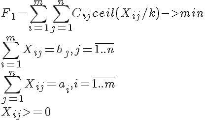
where X is the transportation matrix, i.e. optimized parameter, and ceil - rounding up to the nearest integer.
In addition, we introduce into consideration:
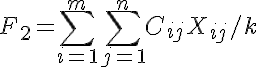
First, we solve the classical transport problem with F2-> min. The obtained value of F2 is the lower bound for F1 on the set of admissible values. Remember the value of F2_save: = F2. We find the value of F1 with the resulting solution X and remember it F1_save = F1. If F1_save == ceil (F2_save), then X is the solution you are looking for, otherwise go further.
F1 can be reduced only by decreasing the basis components of Xto the nearest multiple k values, therefore, we will construct (the branch and bound method) a tree of solutions to problems with additional restrictions. The top of the tree is the solution already received. Each next tier of the tree is constructed as follows: for each basis component (xij) equal to some non-multiple k value (z), we solve the classical transport problem F2-> min with the additional constraint xij = [z / k] * k ([x] Is the integer part of x) (see PS). If for the obtained solution F1= F1_save, then we do not continue this branch. If F1 == ceil (F2_save), then the resulting X is the desired solution, otherwise go further. Thus, we obtain a decision tree, each branch of which ends if ceil (F2)> = F1_save on the sheet of this branch, or if all components from the basis are multiples of k, or if the problem did not have a solution at all. The plan corresponding to that obtained after building the F1_save tree is optimal.
PS Adding a constraint is not necessary to solve the problem again. You can, for example, go through all the possible F1-decreasing cycles and choose the optimal one among them. Or use the methods of the dual simplex method.
Example
Consider the algorithm in a very simple example. Let k = 3, C = {{2,2}, {4,5}}, a = {2,3}, b = {2,3}. So the top of the tree is the solution of such a transport problem with the objective function F2:
0) X = {{0,2}, {2,1}}, F2 (X) ~ = 5.67, F1 (X) = 2 + 4 + 5 = eleven.
F2_save: = 5.67, F1_save: = 11
since ceil (5.67) <11 we go further - we build the next tier of the tree:
1.1) add the condition x12 == 0 to the problem being solved at node 0 and solve it again.
X = {{2.0}, {0.3}}, F2 (X) ~ = 6.35, F1 (X) = 2 + 5 = 7.
because F1
because ceil (F2)> = F1_save (7> = 7), then we do not continue this branch
since F1> ceil (F2_save) we go further (maybe there is a better solution), the branch does not continue, but the tier is not finished yet.
1.2) add the condition x21 == 0 to the problem being solved in node 0 and solve it again.
X = {{2.0}, {0.3}}, F2 (X) ~ = 6.35, F1 (X) = 2 + 5 = 7.
because F1 == F1_save (7 == 7), then F1_save does not change
since ceil (F2)> = F1_save (7> = 7), then we do not continue this branch
since F1> ceil (F2_save) we go further (maybe there is a better solution), the branch does not continue, but the tier is not finished yet.
1.3) add the condition x22 == 0 to the problem being solved in node 0 and solve it again. Such a problem has no solution => and we do not continue this branch.
There are no more basic components left (the tier is finished) and there is no need to continue the branches (pointless, we won’t get a better solution), then the tree is built. F1_save == 7 is our minimum cost. A plan corresponding to them (he is the answer) X = {{2,0}, {0,3}}
A year ago, on the third
course as one of the laboratory work on the course "Optimization Methods" I was asked to implement a solution to the transport problem, but with one small condition: transportation occurs in batches. This means that now, unlike the classic production, the transportation of a consignment of goods (eg 10 pieces) is paid, and even if you need to transport 11 pieces, you will pay for two lots (11 pieces will not fit into one trailer). It would seem a minor addition, but how to solve the problem now, and at least how to formalize it? As a student of the Department of Applied Mathematics, I was not used to the fact that the great google.ru did not know something, but what was my surprise when neither his older brother, the English-speaking google, nor the darkness of the books on optimization theory that I had been able to answer this question.I want to say right away - I do not pretend to use the Fields Award with my algorithm. I do not offer anything supernatural, but for those who are just starting to solve such a problem, I can help a little.
Let C be the payment matrix, a is the vector of cargo stocks, b is the vector of demand for cargo, k is the number of goods in a batch. We will consider the following formalization:
where X is the transportation matrix, i.e. optimized parameter, and ceil - rounding up to the nearest integer.
In addition, we introduce into consideration:
First, we solve the classical transport problem with F2-> min. The obtained value of F2 is the lower bound for F1 on the set of admissible values. Remember the value of F2_save: = F2. We find the value of F1 with the resulting solution X and remember it F1_save = F1. If F1_save == ceil (F2_save), then X is the solution you are looking for, otherwise go further.
F1 can be reduced only by decreasing the basis components of Xto the nearest multiple k values, therefore, we will construct (the branch and bound method) a tree of solutions to problems with additional restrictions. The top of the tree is the solution already received. Each next tier of the tree is constructed as follows: for each basis component (xij) equal to some non-multiple k value (z), we solve the classical transport problem F2-> min with the additional constraint xij = [z / k] * k ([x] Is the integer part of x) (see PS). If for the obtained solution F1
PS Adding a constraint is not necessary to solve the problem again. You can, for example, go through all the possible F1-decreasing cycles and choose the optimal one among them. Or use the methods of the dual simplex method.
Example
Consider the algorithm in a very simple example. Let k = 3, C = {{2,2}, {4,5}}, a = {2,3}, b = {2,3}. So the top of the tree is the solution of such a transport problem with the objective function F2:
0) X = {{0,2}, {2,1}}, F2 (X) ~ = 5.67, F1 (X) = 2 + 4 + 5 = eleven.
F2_save: = 5.67, F1_save: = 11
since ceil (5.67) <11 we go further - we build the next tier of the tree:
1.1) add the condition x12 == 0 to the problem being solved at node 0 and solve it again.
X = {{2.0}, {0.3}}, F2 (X) ~ = 6.35, F1 (X) = 2 + 5 = 7.
because F1
since F1> ceil (F2_save) we go further (maybe there is a better solution), the branch does not continue, but the tier is not finished yet.
1.2) add the condition x21 == 0 to the problem being solved in node 0 and solve it again.
X = {{2.0}, {0.3}}, F2 (X) ~ = 6.35, F1 (X) = 2 + 5 = 7.
because F1 == F1_save (7 == 7), then F1_save does not change
since ceil (F2)> = F1_save (7> = 7), then we do not continue this branch
since F1> ceil (F2_save) we go further (maybe there is a better solution), the branch does not continue, but the tier is not finished yet.
1.3) add the condition x22 == 0 to the problem being solved in node 0 and solve it again. Such a problem has no solution => and we do not continue this branch.
There are no more basic components left (the tier is finished) and there is no need to continue the branches (pointless, we won’t get a better solution), then the tree is built. F1_save == 7 is our minimum cost. A plan corresponding to them (he is the answer) X = {{2,0}, {0,3}}